
EY Data Challenge: Coastal Infrastructure Damage Detection using Computer Vision
Coastal Infrastructure Damage Detection using YOLO
By: Jorge Solis, Jo-anne Bantugon, Karla Banal, Marcio Pineda, Italo Hidalgo
Hult International Business School
Jupyter notebook and dataset for this analysis can be found here: Portfolio
Introduction to the Business Challenge
The EY Open Science Data Challenge tasked us with creating a machine learning model to identify and classify coastal infrastructure damage caused by natural disasters. The challenge focuses on analyzing satellite images of San Juan, Puerto Rico, before and after Hurricane Maria. The model categorizes the damage into four labels: damaged residential, damaged commercial, undamaged residential, and undamaged commercial. This project aims to aid in rapid damage assessment and efficient resource allocation for disaster response.
Methodology
The project is divided into several parts:
- Data Collection: Satellite images from NASA and labeled images from Roboflow.
- Data Preprocessing: Conversion and preparation of images and labels.
- Model Training: Using YOLO for object detection and classification.
- Model Evaluation: Evaluating the model’s performance using Mean Average Precision (mAP).
Key Knowledge
Located in the northeastern Caribbean, Puerto Rico is part of the “hurricane belt”. The island’s location puts it directly in the path of tropical storms and hurricanes that form in the Atlantic Ocean. Hurricane Maria made landfall in Puerto Rico in September 2017, with sustained winds as high as 155 mph, which was barely below the Category 5 threshold. This natural event caused considerable damage to the island’s infrastructure. The entire island was affected by uprooted trees, power lines pulled down, and residential and commercial roofs being destroyed (Scott, 2018).
In line with the above, we will analyze the Normalized Difference Vegetation Index (NDVI) to evaluate the health of vegetation pre and post storm. Moreover, the use deep learning model such as YOLO (You Only Look Once) for object detection and rapid analysis to assess infrastructure damage after hurricanes will be employed. This is crucial for efficient resource allocation and effective response in disasters’ immediate aftermath. The integration of these technologies ensures that responses are more targeted and that resources are optimally used, which is crucial for areas like Puerto Rico that are frequently in the path of hurricanes.
Top Three Actionable Insights
-
Housing Structure: Housing structures in Old San Juan, which is near the coastal line, are old century houses made of cobblestones or reinforced concrete with either flat roofs and or shingle roofings. The buildings were also erected near each other making them sturdier rather than stand-alone houses or buildings. While the most damaged areas by hurricane happened in rural areas where houses or buildings are more scattered, stand-alone and mostly made out of lightweight materials. One way to lessen the effect of hurricanes on buildings, be it commercial or residential, is by getting people to build more hurricane-proof buildings especially in the rural areas.
-
Emergency / Evacuation Plan: The government must identify shelters and broadcast them in advance, so that people can plan their route to safety. Each house must be equipped with a Basic-Disaster kit or emergency supplies like food, water, medicine, power supplies that will last the whole family for days while waiting for rescue (OSHA). Constant education to the people of San Juan, Puerto Rico on the evacuation plan in case a hurricane hits the country again is essential.
-
Insurance Plan: When Hurricane Maria hit San Juan, Puerto Rico, it uncovered that only a small percentage of the population’s homes were insured. The biggest takeaway from this disaster was the importance of getting homes insured, as it wouldn’t be as costly as rebuilding your home or office buildings out of your own pockets (FEMA).
Part I: Pre- and Post-Event NDVI Analysis
Visualization 01: Accessing Satellite Data
Defining the Area of Interest
# Define the bounding box for the selected region
min_lon = -66.19385887
min_lat =  18.27306794
max_lon = -66.069299
max_lat =  18.400288

# setting geographic boundary
bounds = (min_lon, min_lat, max_lon, max_lat)

# setting time window surrounding the storm landfall on September 20, 2017
time_window = "2017-04-08/2017-10-31"

# calculating days in time window
print(date(2017, 10, 31) - date(2017, 4, 8 ))

# connecting to the planetary computer
stac = pystac_client.Client.open("https://planetarycomputer.microsoft.com/api/stac/v1")

# seaching for data
search = stac.search(collections = ["sentinel-2-l2a"], bbox = bounds, datetime = time_window)
items = list(search.get_all_items())

# summarizing results
print('This is the number of scenes that touch our region:',len(items))

# Use of Open Data Cube (ODC) for managing and analyzing geospatial data
xx = stac_load(
    items,
    bands = ["red", "green", "blue", "nir", "SCL"],
    crs = "EPSG:4326",
    resolution = scale,
    chunks = {"x": 2048, "y": 2048},
    dtype = "uint16",
    patch_url = pc.sign,
    bbox = bounds
)
Visualization 01: Viewing RGB (real color) images from the time series
NDVI Change Product
# running comparison
ndvi_clean = NDVI(cleaned_data)

# calculating difference
ndvi_pre = ndvi_clean.isel(time = first_time)
ndvi_post = ndvi_clean.isel(time = second_time)
ndvi_anomaly = ndvi_post - ndvi_pre

# plotting NDVI anomaly
plt.figure(figsize = (6,10))
ndvi_anomaly.plot(vmin = -0.2, vmax=0.0, cmap = Reds_reverse, add_colorbar=False)
plt.title("NDVI Anomaly")
plt.xlabel("Longitude")
plt.ylabel("Latitude")
plt.show()
Output:
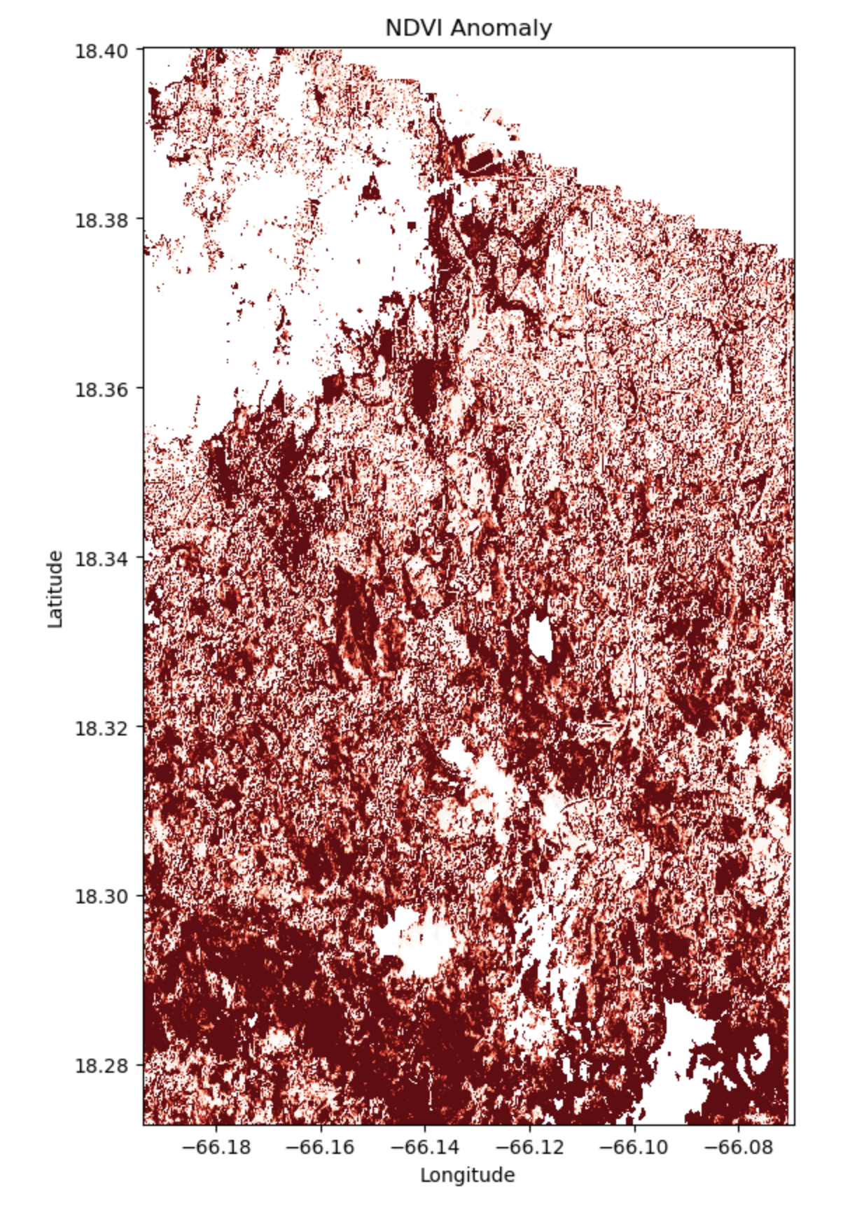
Analysis (Visualization 01)
The forest area shows varying degrees of vegetation change after Hurricane María. The darker red regions indicate severe damage, likely due to high winds, tree fall, and extensive defoliation. Lighter red areas suggest moderate stress or partial vegetation loss, with potential for quicker recovery. These variations underscore the need for targeted recovery efforts and comprehensive disaster preparedness strategies.
Visualization 02: Accessing Satellite Data
# Define the bounding box for the selected region
min_lon = -66.19385887
min_lat =  18.27306794
max_lon = -66.08007533
max_lat =  18.48024350

# setting geographic boundary
bounds = (min_lon, min_lat, max_lon, max_lat)

# setting time window surrounding the storm landfall on September 20, 2017
time_window = "2017-04-08/2017-11-30"

# calculating days in time window
print(date(2017, 11, 1) - date(2017, 4, 1 ))

# connecting to the planetary computer
stac = pystac_client.Client.open("https://planetarycomputer.microsoft.com/api/stac/v1")

# seaching for data
search = stac.search(collections = ["sentinel-2-l2a"], bbox = bounds, datetime = time_window)
items = list(search.get_all_items())

# summarizing results
print('This is the number of scenes that touch our region:',len(items))

# Use of Open Data Cube (ODC) for managing and analyzing geospatial data
xx = stac_load(
    items,
    bands = ["red", "green", "blue", "nir", "SCL"],
    crs = "EPSG:4326",
    resolution = scale,
    chunks = {"x": 2048, "y": 2048},
    dtype = "uint16",
    patch_url = pc.sign,
    bbox = bounds
)
NDVI Change Product
# running comparison
ndvi_clean = NDVI(cleaned_data)

# calculating difference
ndvi_pre = ndvi_clean.isel(time = first_time)
ndvi_post = ndvi_clean.isel(time = second_time)
ndvi_anomaly = ndvi_post - ndvi_pre

# plotting NDVI anomaly
plt.figure(figsize = (6,10))
ndvi_anomaly.plot(vmin = -0.2, vmax=0.0, cmap = Reds_reverse, add_colorbar=False)
plt.title("NDVI Anomaly")
plt.xlabel("Longitude")
plt.ylabel("Latitude")
plt.show()
Output:
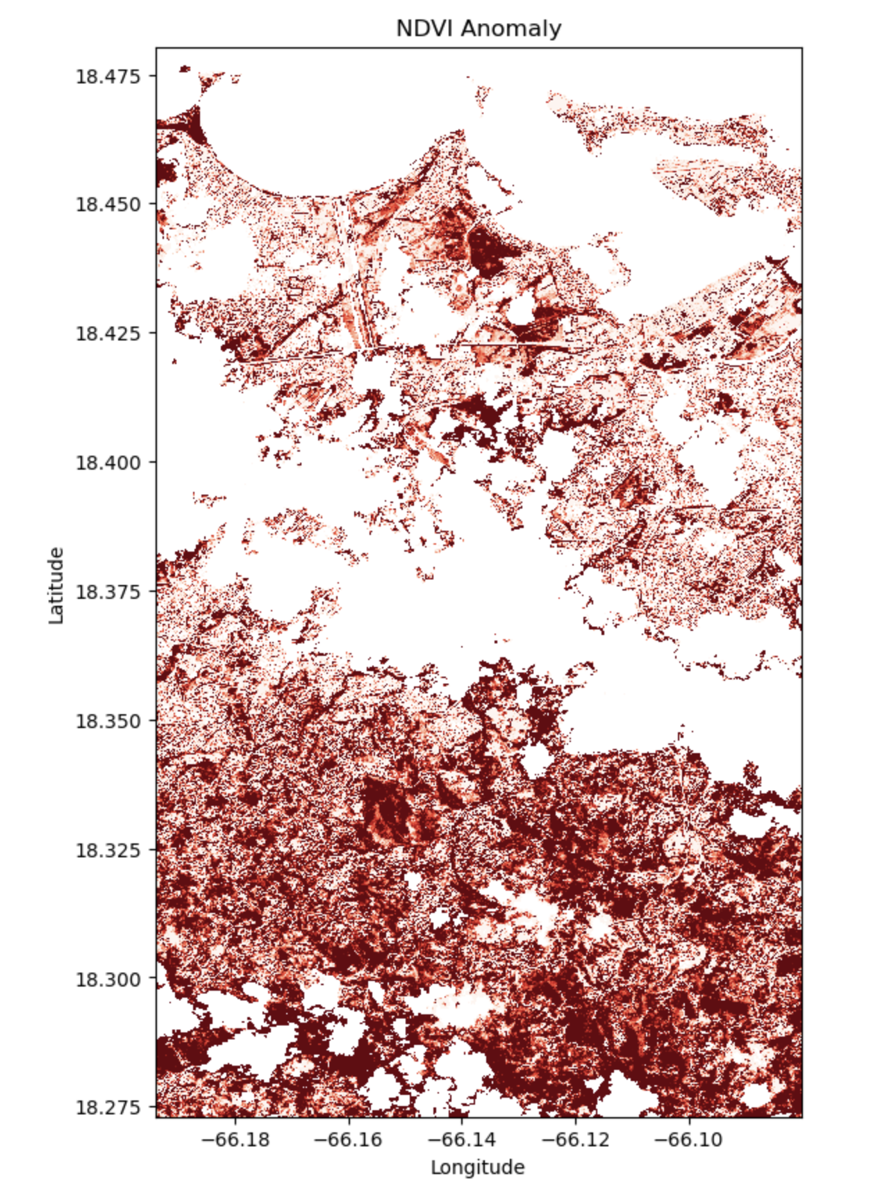
Analysis (Visualization 02)
The dark red zones reflect acute vegetative destruction, hinting at the harsh conditions endured. Lighter reds and pinks signal less impacted areas that might recover more quickly. These findings highlight the need for targeted restoration efforts and ongoing ecological tracking.
Visualization 03: Accessing Satellite Data
# Define the bounding box for the selected region
min_lon = -66.1327369
min_lat =  18.4063942
max_lon = -66.0673603
max_lat =  18.4784524

# setting geographic boundary
bounds = (min_lon, min_lat, max_lon, max_lat)

# setting time window surrounding the storm landfall on September 20, 2017
time_window = "2017-04-01/2017-11-01"

# calculating days in time window
print(date(2017, 11, 1) - date(2017, 4, 1 ))

# connecting to the planetary computer
stac = pystac_client.Client.open("https://planetarycomputer.microsoft.com/api/stac/v1")

# seaching for data
search = stac.search(collections

 = ["sentinel-2-l2a"], bbox = bounds, datetime = time_window)
items = list(search.get_all_items())

# summarizing results
print('This is the number of scenes that touch our region:',len(items))

# Use of Open Data Cube (ODC) for managing and analyzing geospatial data
xx = stac_load(
    items,
    bands = ["red", "green", "blue", "nir", "SCL"],
    crs = "EPSG:4326",
    resolution = scale,
    chunks = {"x": 2048, "y": 2048},
    dtype = "uint16",
    patch_url = pc.sign,
    bbox = bounds
)
NDVI Change Product
# running comparison
ndvi_clean = NDVI(cleaned_data)

# calculating difference
ndvi_pre = ndvi_clean.isel(time = first_time)
ndvi_post = ndvi_clean.isel(time = second_time)
ndvi_anomaly = ndvi_post - ndvi_pre

# plotting NDVI anomaly
plt.figure(figsize = (6,10))
ndvi_anomaly.plot(vmin = -0.2, vmax=0.0, cmap = Reds_reverse, add_colorbar=False)
plt.title("NDVI Anomaly")
plt.xlabel("Longitude")
plt.ylabel("Latitude")
plt.show()
Output:
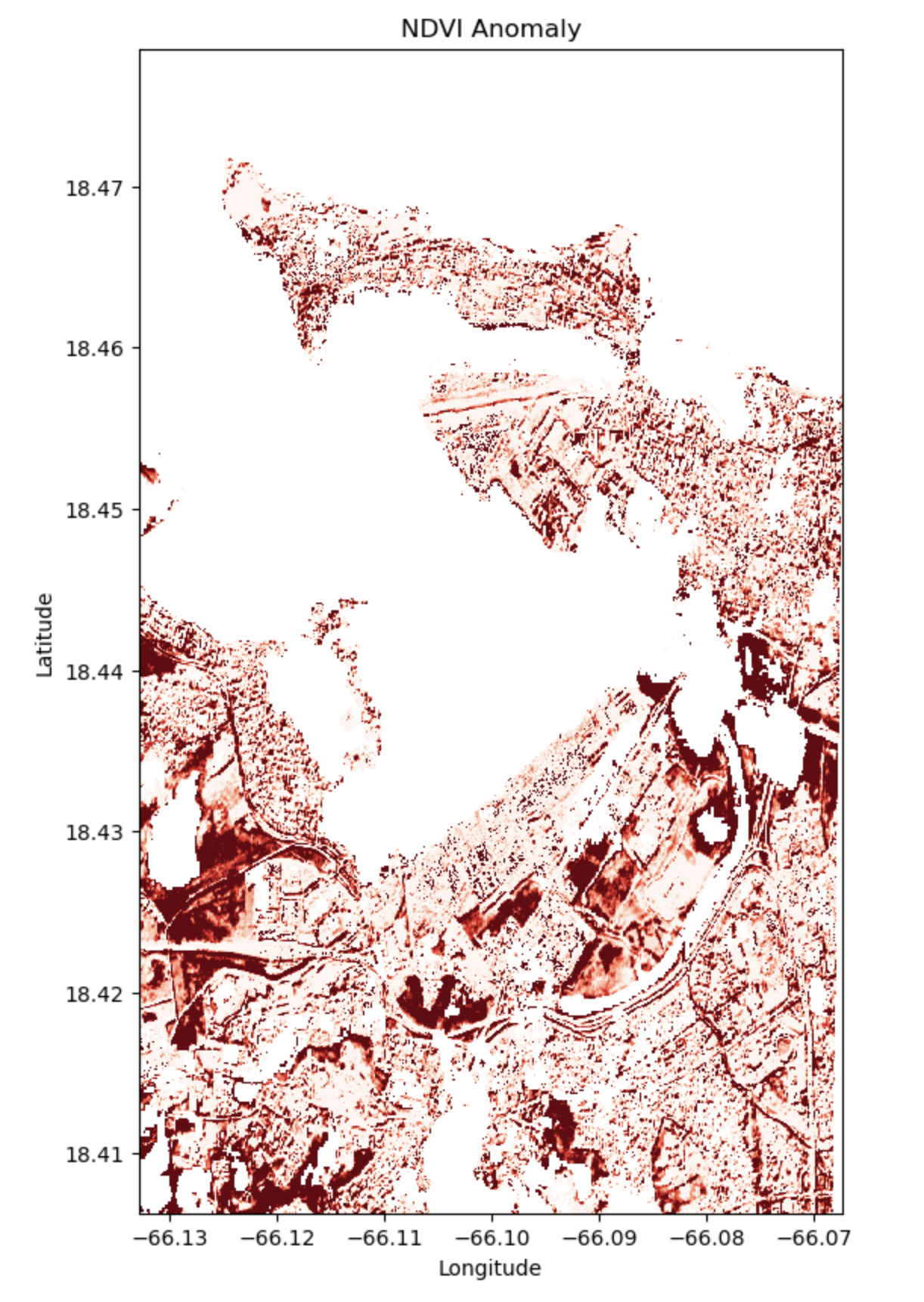
Analysis (Visualization 03)
The visualization highlights striking contrasts in vegetation health with dark red areas indicating substantial damage, likely due to strong winds and rain near the coastal area for urban and suburban neighborhoods. Paler reds suggest areas of moderate impact, with prospects for a more rapid recovery. The insights call for targeted reconstruction and strategic planning for similar future events.
Part II: Object Detection and Model Building
Generating Training and Testing Data along with the Configuration File
!labelme2yolo --json_dir "./labelme_json_dir/"
Model Building and Model Training
# Loading the model
model = YOLO('yolov8n.pt')
# Display model information (optional)
model.info()
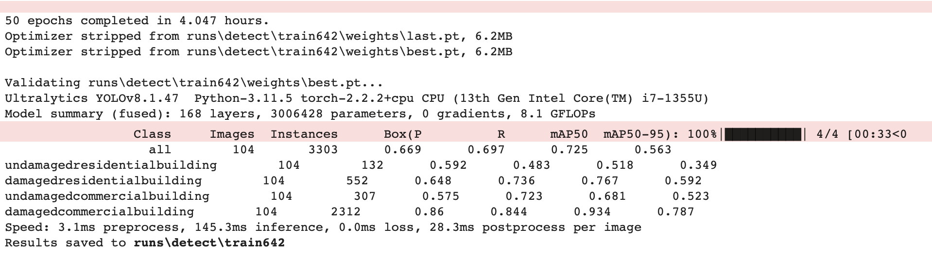
# Train the model on the dataset for 50 epochs
results = model.train(data = "./datasets/dataset.yaml", epochs = 50, imgsz = 512)
Output:
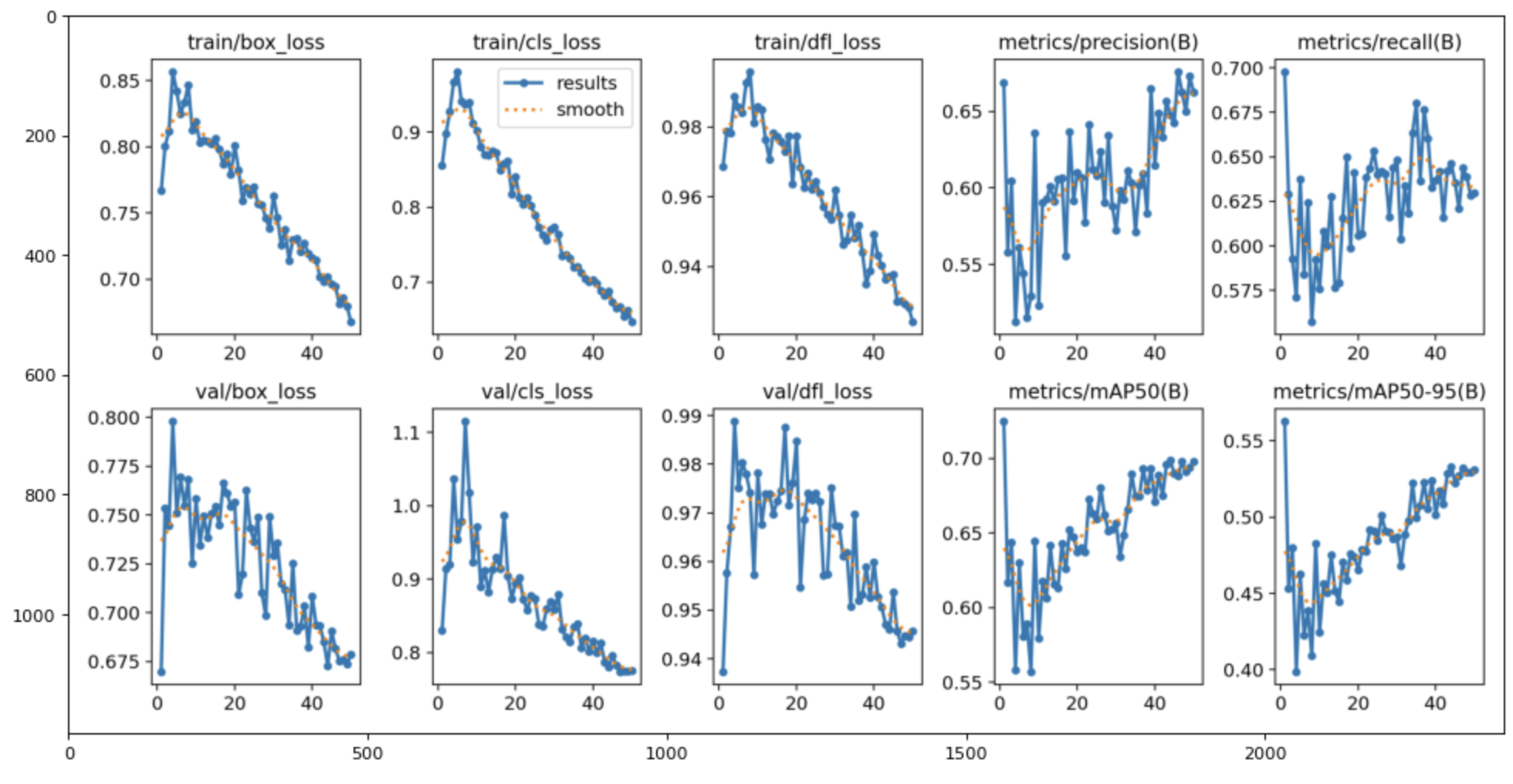
Model Evaluation
%matplotlib inline

figure(figsize=(15, 10), dpi=80)
# reading the image
results = img.imread('./runs/detect/train642/results.png')

# displaying the image
plt.imshow(results)
plt.show()
Output:
Part III: Model Analysis
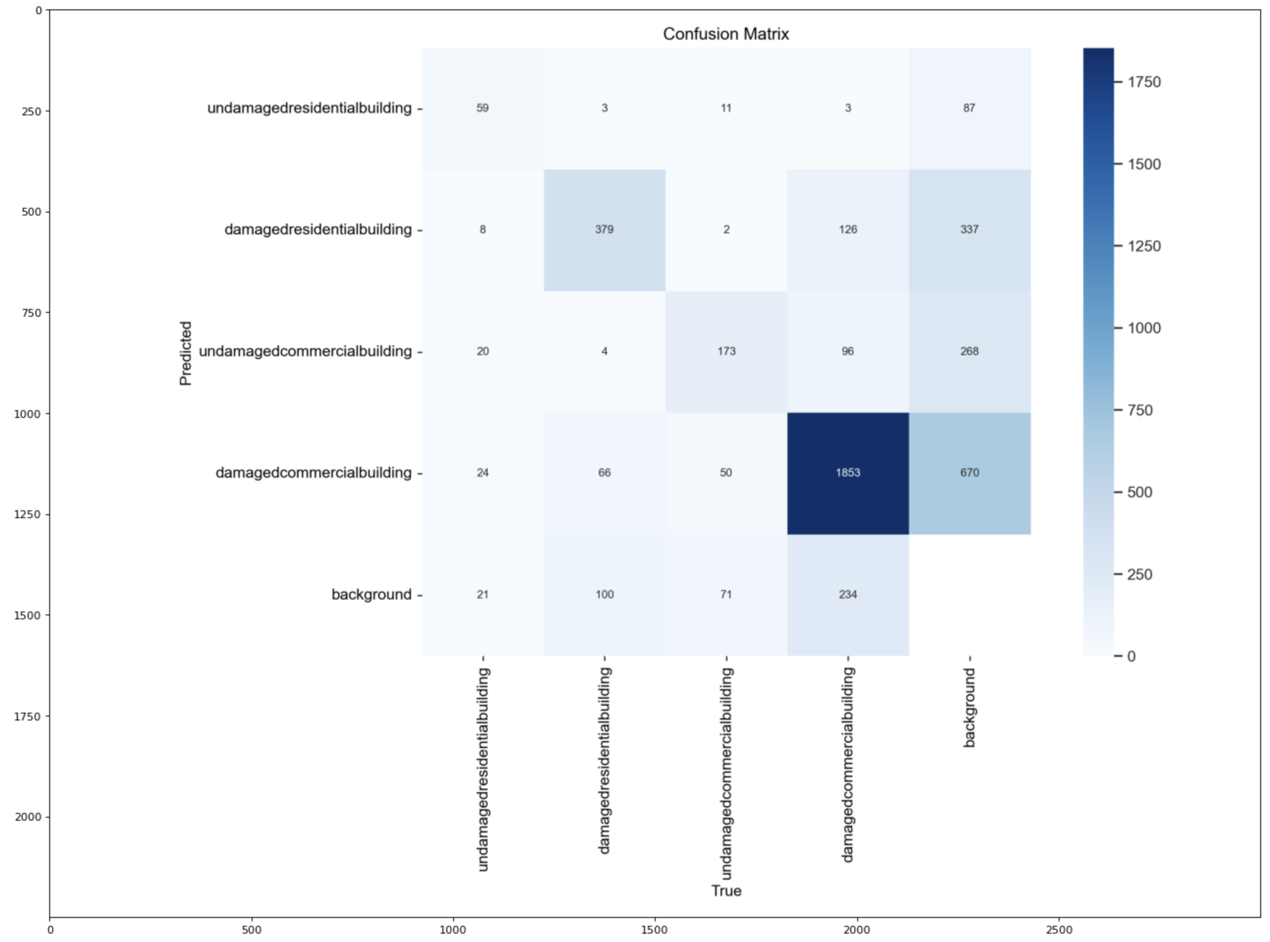
Confusion Matrix
figure(figsize=(20,15), dpi=80)

# reading the image
cf = img.imread('./runs/detect/train642/confusion_matrix.png')

# displaying the image
plt.imshow(cf)
plt.show()
Output:
Converting Confusion Matrix to One Class
Class 1 Undamaged residential buildings
# Confusion Matrix for Class 1 (2x2)
confusion_matrix_one = np.array([ [59, 104],
                                  [73,  4429] ] )

# Select rows and columns corresponding to class 1
class_index = 0
tn_1 = confusion_matrix_one[class_index, class_index]
fp_1 = confusion_matrix_one[:, class_index].sum() - tp_1
fn_1 = confusion_matrix_one[class_index, :].sum() - tp_1
tp_1 = confusion_matrix_one.sum() - tn_1 - fp_1 - fn_1

# Construct one-vs-all confusion matrix for class 1
class_one = np.array([[tp_1, fp_1],
                      [fn_1, tn_1]])

print("Confusion Matrix for Class 1 (undamaged residential building)")

# Unpacking the one-vs-all confusion matrix for Class 1
tn_1, fp_1, fn_1, tp_1 = class_one.ravel()

# Printing each result one-by-one
print(f"""
True Positives: {tp_1}
False Positives: {fp_1}
True Negatives: {tn_1}
False Negatives: {fn_1}
""")

# Calculate precision and recall for Class 1 (undamaged residential building)
precision_1 = tp_1 / (tp_1 + fp_1)
recall_1 = tp_1 / (tp_1 + fn_1)

print(f"Precision for Class 1: {precision_1:.4f}")
print(f"Recall for Class 1: {recall_1:.4f}")
Confusion Matrix for Class 1 (undamaged residential building)
- True Positives: 59
- False Positives: 73
- True Negatives: 4429
-
False Negatives: 104
- Precision for Class 1: 0.4470
- Recall for Class 1: 0.3620
Class 2 Damaged residential buildings
# Confusion Matrix for Class 2 (2x2)
confusion_matrix_two = np.array([ [379, 473],
                                  [173,  3640] ] )

# Select rows and columns corresponding to class 2
class_index = 0
tn_2 = confusion_matrix_two[class_index, class_index]
fp_2 = confusion_matrix_two[:, class_index].sum() - tp_2
fn_2 = confusion_matrix_two[class_index, :].sum() - tp_2
tp_2 = confusion_matrix_two.sum() - tn_2 - fp_2 - fn_2

# Construct one-vs-all confusion matrix for class 2
class_two = np.array([[tp_2, fp_2],
                      [fn_2, tn_2]])

print("Confusion Matrix for Class 2 (damaged residential building)")

# Unpacking the one-vs-all confusion matrix for Class 2
tn_2, fp_2, fn_2, tp_2 = class_two.ravel()

# Printing each result one-by-one
print(f"""
True Positives: {tp_2}
False Positives: {fp_2}
True Negatives: {tn_2}
False Negatives: {fn_2}
""")

# Calculate precision and recall for Class 2 (damaged residential buildings)
precision_2 = tp_2 / (tp_2 + fp_2)
recall_2 = tp_2 / (tp_2 + fn_2)

print(f"Precision for Class 2: {precision_2:.4f}")
print(f"Recall for Class 2: {recall_2:.4f}")
Confusion Matrix for Class 2 (damaged residential building)
- True Positives: 379
- False Positives: 173
- True Negatives: 3640
-
False Negatives: 473
- Precision for Class 2: 0.6866
- Recall for Class 2: 0.4448
Class 3 Undamaged commercial building
# Confusion Matrix for Class 3 (2x2)
confusion_matrix_three = np.array([ [173, 388],
                                    [134, 3970] ] )

# Select rows and columns corresponding to class 3
class_index = 0
tn_3 = confusion_matrix_three[class_index, class_index]
fp_3 = confusion_matrix_three[:, class_index].sum() - tp_3
fn_3 = confusion_matrix_three[class_index, :].sum() - tp_3
tp_3 = confusion_matrix_three.sum() - tn_3 - fp_3 - fn_3

# Construct one-vs-all confusion matrix for class 3
class_three = np.array([[tp_3, fp_3],
                      [fn_3, tn_3]])

print("Confusion Matrix for Class 3 (undamaged commercial building)")

# Unpacking the one-vs-all confusion matrix for Class 3
tn_3, fp_3, fn_3, tp_3 = class_three.ravel()

# Printing each result one-by-one
print(f"""
True Positives: {tp_3}
False Positives: {fp_3}
True Negatives: {tn_3}
False Negatives: {fn_3}
""")

# Calculate precision and recall for Class 3
precision_3 = tp_3 / (tp_3 + fp_3)
recall_3 = tp_3 / (tp_3 + fn_3)

print(f"Precision for Class 3: {precision_3:.4f}")
print(f"Recall for Class 3: {recall_3:.4f}")
Confusion Matrix for Class 3 (undamaged commercial building)
- True Positives: 173
- False Positives: 134
- True Negatives: 3970
-
False Negatives: 388
- Precision for Class 3: 0.5635
- Recall for Class 3: 0.3084
Class 4 Damaged commercial building
# Confusion Matrix for Class 4 (2x2)
confusion_matrix_four = np.array([ [1853, 810],
                                    [459, 1543] ] )

# Select rows and columns corresponding to class 4
class_index = 0
tn_4 = confusion_matrix_four[class_index, class_index]
fp_4 = confusion_matrix_four[:, class_index].sum() - tp_4
fn_4 = confusion_matrix_four[class_index, :].sum() - tp_4
tp_4 = confusion_matrix_four.sum() - tn_4 - fp_4 - fn_4

# Construct one-vs-all confusion matrix for class 4
class_four = np.array([[tp_4, fp_4],
                      [fn_4, tn_4]])

print("Confusion Matrix for Class 4 (damaged commercial building)")

# Unpacking the one-vs-all confusion matrix for Class 4
tn_4, fp_4, fn_4, tp_4 = class_four.ravel()

# Printing each result one-by-one
print(f"""
True Positives: {tp_4}
False Positives: {fp_4}
True Negatives: {tn_4}
False Negatives: {fn_4}
""")

# Calculate precision and recall for Class 4
precision_4 = tp_4 / (tp_4 + fp_4)
recall_4 = tp_4 / (tp_4 + fn_4)

print(f"Precision for Class 4: {precision_4:.4f}")
print(f"Recall for Class 4: {recall_4:.4f}")
Confusion Matrix for Class 4 (damaged commercial building)
- True Positives: 1853
- False Positives: 459
- True Negatives: 1543
-
False Negatives: 810
- Precision for Class 2: 0.8015
- Recall for Class 2: 0.6958
Confusion Matrix Analysis
Undamaged vs. Damaged Commercial Buildings
Between undamaged and damaged commercial buildings, the model shows a notable difference in performance. It exhibits higher precision and recall for identifying damaged commercial buildings compared to undamaged ones. This indicates that model is more adept at correctly classifying damaged commercial buildings while minimizing false positives and false negatives in this category.
Undamaged vs. Damaged Residential Buildings
Similarly, when comparing undamaged and damaged residential buildings, the model demonstrates a similar trend. It performs better in correctly identifying damaged residential buildings, with higher precision and recall scores, suggesting that it is more reliable in distinguishing these structures from undamaged ones.
Overall, the model shows a trend of higher performance in identifying damaged buildings across both residential and commercial categories, with varying levels of precision and recall for each class.
Conclusion
Our team labeled 60 images for both pre- and post-storm scenarios, achieving an mAP of around 0.50. Additionally, we leveraged Open Source Roboflow datasets, which use auto labeling, with the same images. We tried three different labeling approaches and concluded that manual labeling using polygons that outline the shape of the building without background elements yielded highest results compared to using fixed rectangles. Labeling commercial buildings is identifiable since we considered big parking spaces and flat roofings, while for residential buildings, it tends to appear smaller and with a ridge line in roofing.
Given more time, we could explore hybrid approaches of using polygons and fixed rectangles with overlapping, similar to how Roboflow labeled it. This is for further analysis, as our model performance improved after using open-source datasets from Roboflow.
Model results offer insights to NASA, Ernst and Young, and infrastructure sectors, enhancing disaster response using machine learning and deep learning with Sentinel-2 data, promoting resilient communities.
Steps your team would implement/improve if you were given three months to work on this project
Continuously improving the object detection model possibly by using more advanced models for accurate labeling and prediction. Also, considering the size of the buildings, among other features, may enhance its ability to classify damaged and undamaged buildings accurately, leading to better results. Additionally, QGIS offers tools for spatial analysis and feature extraction, allowing for further refinement of object detection algorithms based on building characteristics such as size, shape, and spatial arrangement. Applying advanced pre-processing techniques (sharpening, noise reduction) to improve image clarity. Finally, employing a hybrid approach in manual labeling and using auto-labeling tools to compare results could be beneficial.
Feedback to EY
The team faced several challenges in analyzing images, including the need to enhance image quality for easier annotation and labeling. Blurred or hard-to-identify images pose challenges. Additionally, differences in frame area and angle between pre- and post-images make comparisons difficult. For example, a small building in the pre-image might appear larger in the post-image, potentially affecting model accuracy in labeling buildings correctly. Quality differences, such as clear skies in the pre-image versus cloud cover or shadows in the post-image, limit the selection of suitable images for the model.
References
- Bane, B. (2021, September 22). Artificial Intelligence brings better hurricane predictions. Pacific Northwest National Laboratory. https://www.pnnl.gov/news-media/artificial-intelligence-brings-better-hurricane-predictions
- Find Codes. (n.d.). Codes.iccsafe.org. https://codes.iccsafe.org/codes/puerto-rico
- Grabmeier, J. (2022, October 6). New machine learning model can provide more accurate assessments of hurricane damage for responders. The Ohio State University. https://techxplore.com/news/2022-10-machine-accurate-hurricane.html
- Hosannah, N., Ramamurthy, P., Marti, J., Munoz, J., & González, J. E. (2021). Impacts of Hurricane Maria on land and convection modification over Puerto Rico. Journal of Geophysical Research: Atmospheres, 126, e2020JD032493. https://doi. org/10.1029/2020JD032493
-
Hurricane Preparedness and Response - Preparedness Occupational Safety and Health Administration. (n.d.). www.osha.gov. https://www.osha.gov/hurricane/preparedness - Kundu, R. (2022, August 3). Image Processing: Techniques, Types & Applications [2023]. https://www.v7labs.com/blog/image-processing-guide
- Maayan, G. (2023, September 12). Complete Guide to Image Labeling for Computer Vision. Comet. https://www.comet.com/site/blog/complete-guide-to-image-labeling-for-computer-vision/
- Microsoft Planetary Computer. Landsat Collection 2 Level-2. https://planetarycomputer.microsoft.com/dataset/landsat-c2-l2
- Microsoft Planetary Computer. Sentinel-2 Level-2A. https://planetarycomputer.microsoft.com/dataset/sentinel-2-l2a
- NASA (July 2019). NASA Surveys Hurricane Damage to Puerto Rico’s Forests (Data Viz Version). https://svs.gsfc.nasa.gov/4735/
- PBS Org (March, 2019). Hurricane Maria Devastated Puerto Rico’s Forests at an Unprecedented Rate. https://www.pbs.org/wgbh/nova/article/hurricane-maria-devastated-puerto-ricos-forests-at-an-unprecedented-rate/
- Pérez Valentín, J. M., & Müller, M. F.(2020). Impact of Hurricane Maria onbeach erosion in Puerto Rico: Remotesensing and causal inference.Geophysical Research Letters,47,e2020GL087306. https://doi.org/10.1029/2020GL087306Received
- Protective Actions Research. (2024). Fema.gov. https://community.fema.gov/ProtectiveActions/s/article/Hurricane-Review-Your-Insurance
- Roboflow User (um). tes1 Image Dataset. https://universe.roboflow.com/um-w3o1a/tes1-mjea9/dataset/3. Retrieved 24Apr2023
- Scott, M. (2018, August 1). Hurricane Maria’s devastation of Puerto Rico. https://www.climate.gov/news-features/understanding-climate/hurricane-marias-devastation-puerto-rico
- Shorten, C., Khoshgoftaar, T.M. (2019, July 6). A survey on Image Data Augmentation for Deep Learning. J Big Data 6, 60 (2019). https://doi.org/10.1186/s40537-019-0197-0
- USGS. Landsat Collection 2 Quality Assessment Bands. https://www.usgs.gov/landsat-missions/landsat-collection-2-quality-assessment-bands