Predicting Bike Rentals in Chicago Using Machine Learning

24 minute read

Bike Rental Demand Forecasting Project

By: Jorge Solis
Hult International Business School

Jupyter notebook and dataset for this analysis can be found here: Portfolio

Introduction

The bike-sharing industry has witnessed exponential growth, with a global market value of approximately $2.8 billion in 2023. Factors such as convenience, sustainability, and the promotion of physical fitness contribute to this surge. Tasked by a major US city, this project aims to develop a machine learning model to predict daily bike rentals and uncover the factors influencing rental demand.

Objective

The objective of this project is to develop a machine learning model to predict the number of bike rentals on a given day, as well as to provide insights into the factors that contribute to bike rental demand. This project was conducted as part of the ‘Computational Data Analytics with Python’ course at Hult International Business School.

The permitted models for this task are:

OLS Linear Regression
Lasso Regression
Ridge Regression
Elastic Net Regression
K-Nearest Neighbors
Decision Tree Regressor

This project was also part of an internal competition on the Kaggle platform at Hult International Business School.

Part I: Imports and Data Check

Importing Libraries

# Importing libraries

# for this template submission
import numpy as np                       # mathematical essentials
import pandas as pd                      # data science essentials
import sklearn.linear_model              # linear models
from sklearn.model_selection import train_test_split # train/test split

# Import additional libraries
import seaborn as sns # enhanced graphical output
import matplotlib.pyplot as plt # essential graphical output
import statsmodels.formula.api as smf # regression modeling

from sklearn.neighbors import KNeighborsRegressor # KNN for Regression
from sklearn.preprocessing import StandardScaler  # standard scaler

from sklearn.tree import DecisionTreeRegressor         # regression trees
from sklearn.tree import plot_tree     
from sklearn.model_selection import RandomizedSearchCV # hyperparameter tuning

# setting pandas print options (optional)
pd.set_option('display.max_rows', 500)
pd.set_option('display.max_columns', 500)
pd.set_option('display.width', 1000)

Importing Data

# Importing data

# Reading modeling data into Python
modeling_data = './datasets/chicago_training_data.xlsx'

# Calling this df_train
df_train = pd.read_excel(io         = modeling_data,
                         sheet_name = 'data',
                         header     = 0,
                         index_col  = 'ID')

# Reading testing data into Python
testing_data = './datasets/test.xlsx'

# Calling this df_test
df_test = pd.read_excel(io         = testing_data,
                        sheet_name = 'data',
                        header     = 0,
                        index_col  = 'ID')

Concatenating Datasets

# Concatenating datasets together for mv analysis and feature engineering
df_train['set'] = 'Not Kaggle'
df_test ['set'] = 'Kaggle'

# Concatenating both datasets together for mv and feature engineering
df_full = pd.concat(objs = [df_train, df_test],
                    axis = 0,
                    ignore_index = False)

# Checking data
df_full.head(n = 5)

# Checking available features
df_full.columns

Setting Response Variable

# Setting response variable
y_variable = 'RENTALS'
df_full_mv = df_full

Part II: Data Preparation

Base Modeling

# Base Modeling

# Information about each variable
df_full.info(verbose = True)

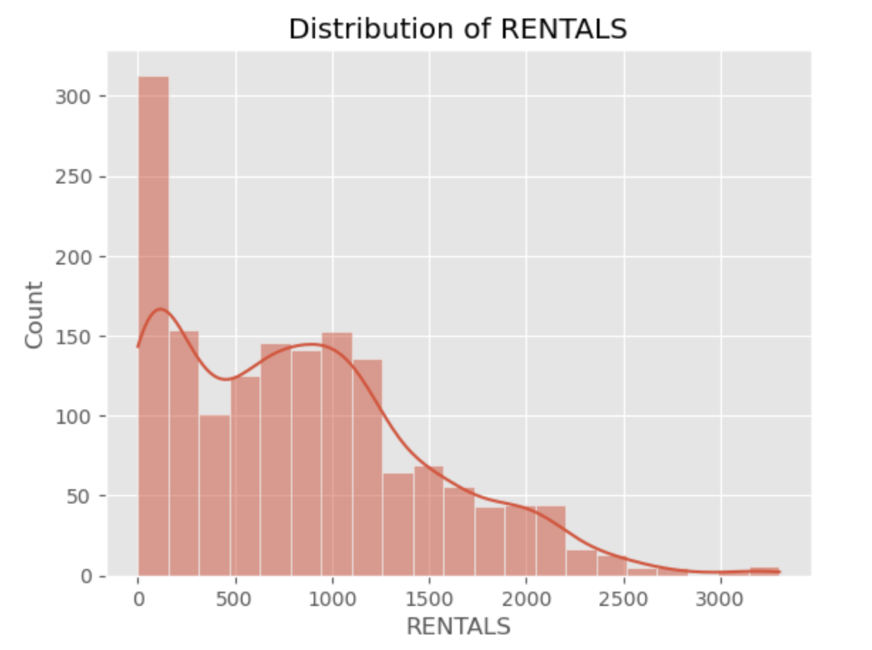
# Developing a histogram using HISTPLOT
sns.histplot(data  = df_train,
         x     = "RENTALS",
         kde   = True)

# Title and axis labels
plt.title(label   = "Distribution of RENTALS")
plt.xlabel(xlabel = "RENTALS") # avoiding using dataset labels
plt.ylabel(ylabel = "Count")

# Displaying the histogram
plt.show()

Output: linearly separable data

data_0 = df_train[df_train.FunctioningDay == 'Yes']
sns.histplot(data  = data_0,
         x     = "RENTALS",
         kde   = True)

# Title and axis labels
plt.title(label   = "Distribution of RENTALS")
plt.xlabel(xlabel = "RENTALS") # avoiding using dataset labels
plt.ylabel(ylabel = "Count")

# Displaying the histogram
plt.show()

sns.lineplot(data = df_train,
            x = 'DateHour',
            y ='RENTALS')

# Title and axis labels
plt.title(label   = "Distribution of RENTALS")
plt.xlabel(xlabel = "RENTALS") # avoiding using dataset labels
plt.ylabel(ylabel = "Count")

# Displaying the histogram
plt.show()

inputs_num = ['Temperature(F)', 'Humidity(%)', 'Wind speed (mph)', 'Visibility(miles)', 'DewPointTemperature(F)', 'Rainfall(in)', 'Snowfall(in)', 'SolarRadiation(MJ/m2)']
plt.style.use('ggplot')
num_bins = 10
data_0 = df_train[df_train.FunctioningDay == 'Yes']

for i in inputs_num:
    n, bins, patches = plt.hist(data_0[i], num_bins, facecolor='blue', alpha=0.5)
    plt.xlabel(i)
    plt.ylabel('Número')
    plt.show()

inputs_num = ['Temperature(F)', 'Humidity(%)', 'Wind speed (mph)', 'Visibility(miles)', 'DewPointTemperature(F)', 'Rainfall(in)', 'Snowfall(in)', 'SolarRadiation(MJ/m2)']
plt.style.use('ggplot')
num_bins = 10
data_1 = df_full[df_full.FunctioningDay == 'Yes']

for i in inputs_num:
    n, bins, patches = plt.hist(data_0[i], num_bins, facecolor='blue', alpha=0.5)
    plt.xlabel(i)
    plt.ylabel('Número')
    plt.show()

# Descriptive statistics for numeric data
df_full_stats = data_0.iloc[ :, 1: ].describe(include = 'number').round(decimals = 2)
df_full_stats

# Developing a correlation matrix
df_full_corr = data_0.corr(method = 'pearson',numeric_only = True)
df_full_corr

# Filtering results to show correlations with Sale_Price
df_full_corr.loc[ : , "RENTALS"].round(decimals = 2).sort_values(ascending = False)

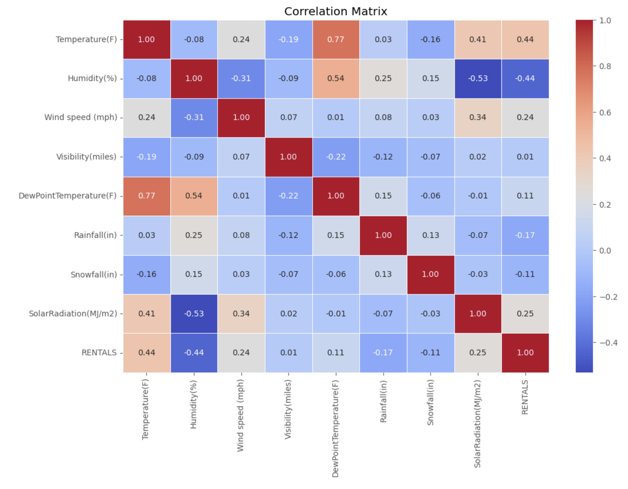
# Plot the correlation matrix using a heatmap
plt.figure(figsize=(12, 8))
sns.heatmap(df_full_corr, 
            annot=True, fmt=".2f", 
            cmap='coolwarm', 
            cbar=True, 
            linewidths=0.5)
plt.title('Correlation Matrix')
plt.show()

Output: linearly separable data

# Setting figure size
fig, ax = plt.subplots(figsize = (9, 6))

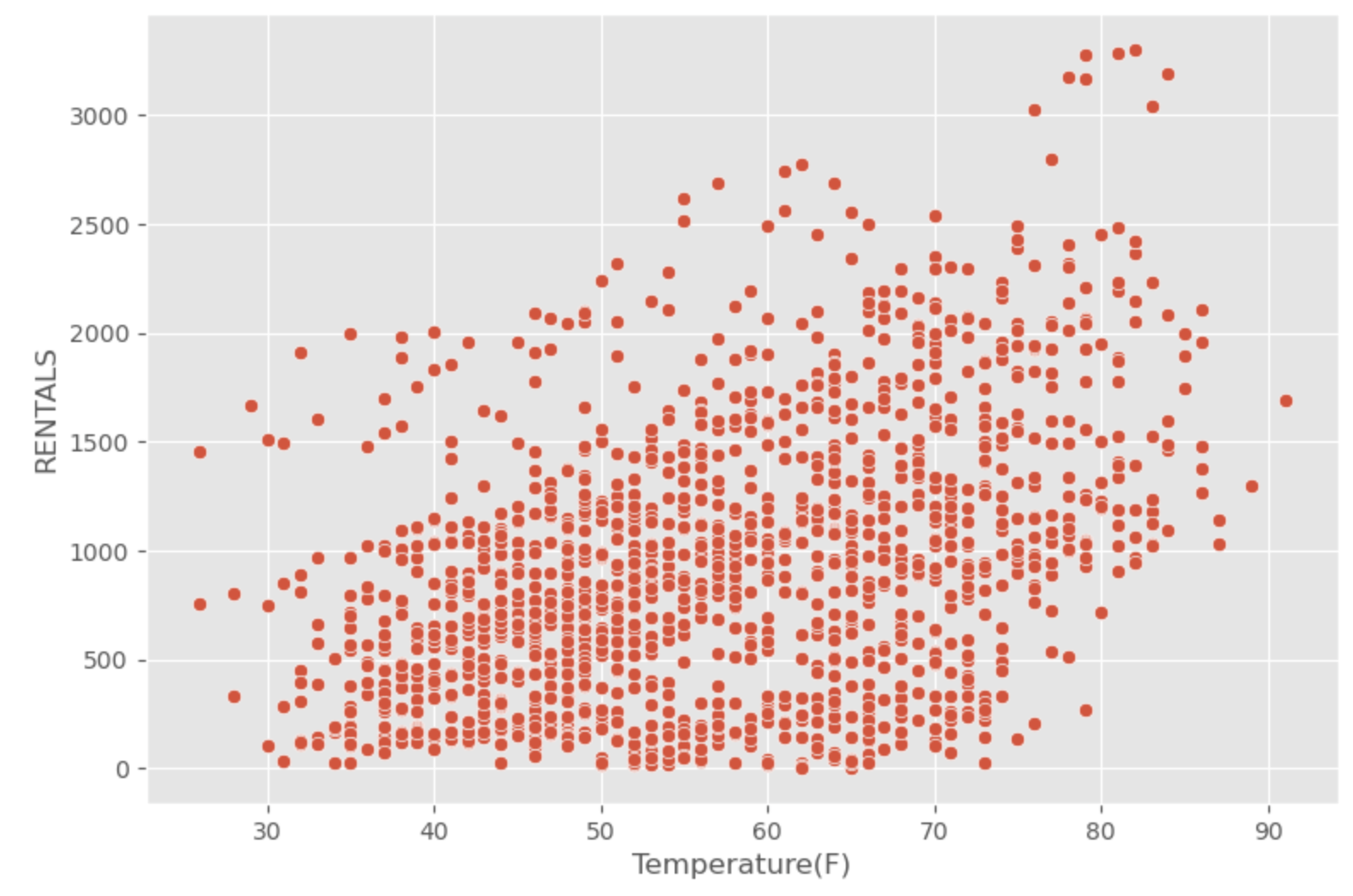
# Developing a scatterplot
sns.scatterplot(x    = "Temperature(F)",
         y    = "RENTALS",
         data = data_0)

# Showing the results
plt.show()

Output: linearly separable data

# Setting figure size
fig, ax = plt.subplots(figsize = (9, 6))

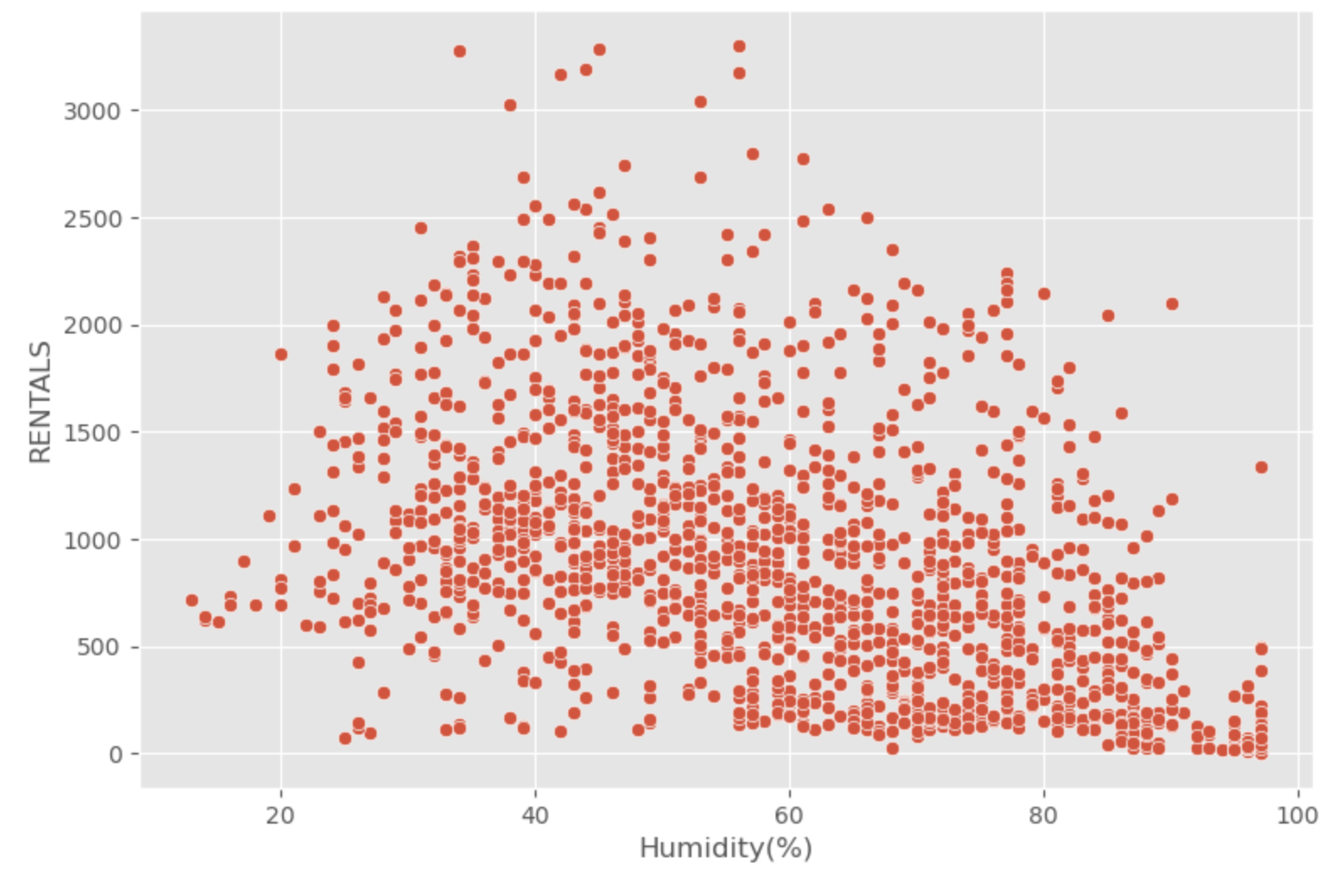
# Developing a scatterplot
sns.scatterplot(x    = "Humidity(%)",
         y    = "RENTALS",
         data = data_0)

# Showing the results
plt.show()

Output: linearly separable data

Missing Value Analysis and Imputation

# Missing Value Analysis and Imputation

df_full.isnull().describe()
df_full.isnull().sum(axis = 0)

df_full.isnull().mean(axis = 0)

# Looping to flag features with missing values
for col in df_full:
    if df_full[col].isnull().astype(int).sum() > 0:
        df_full['m_'+col] = df_full[col].isnull().astype(int)

df_full.columns

df_full = df_full.drop(columns=['m_RENTALS'])
df_full.columns

# Checking results - summing missing value flags
df_full[ ['m_Visibility(miles)', 'm_DewPointTemperature(F)', 'm_SolarRadiation(MJ/m2)'] ].sum(axis = 0)

# Subsetting for mv features
mv_flag_check = df_full[ ['Visibility(miles)'     , 'm_Visibility(miles)',
                          'DewPointTemperature(F)' , 'm_DewPointTemperature(F)',
                          'SolarRadiation(MJ/m2)', 'm_SolarRadiation(MJ/m2)'] ]

# Checking results - feature comparison
mv_flag_check.sort_values(by = ['m_Visibility(miles)', 'm_DewPointTemperature(F)', 'm_SolarRadiation(MJ/m2)'],
                          ascending = False).head(n = 10)

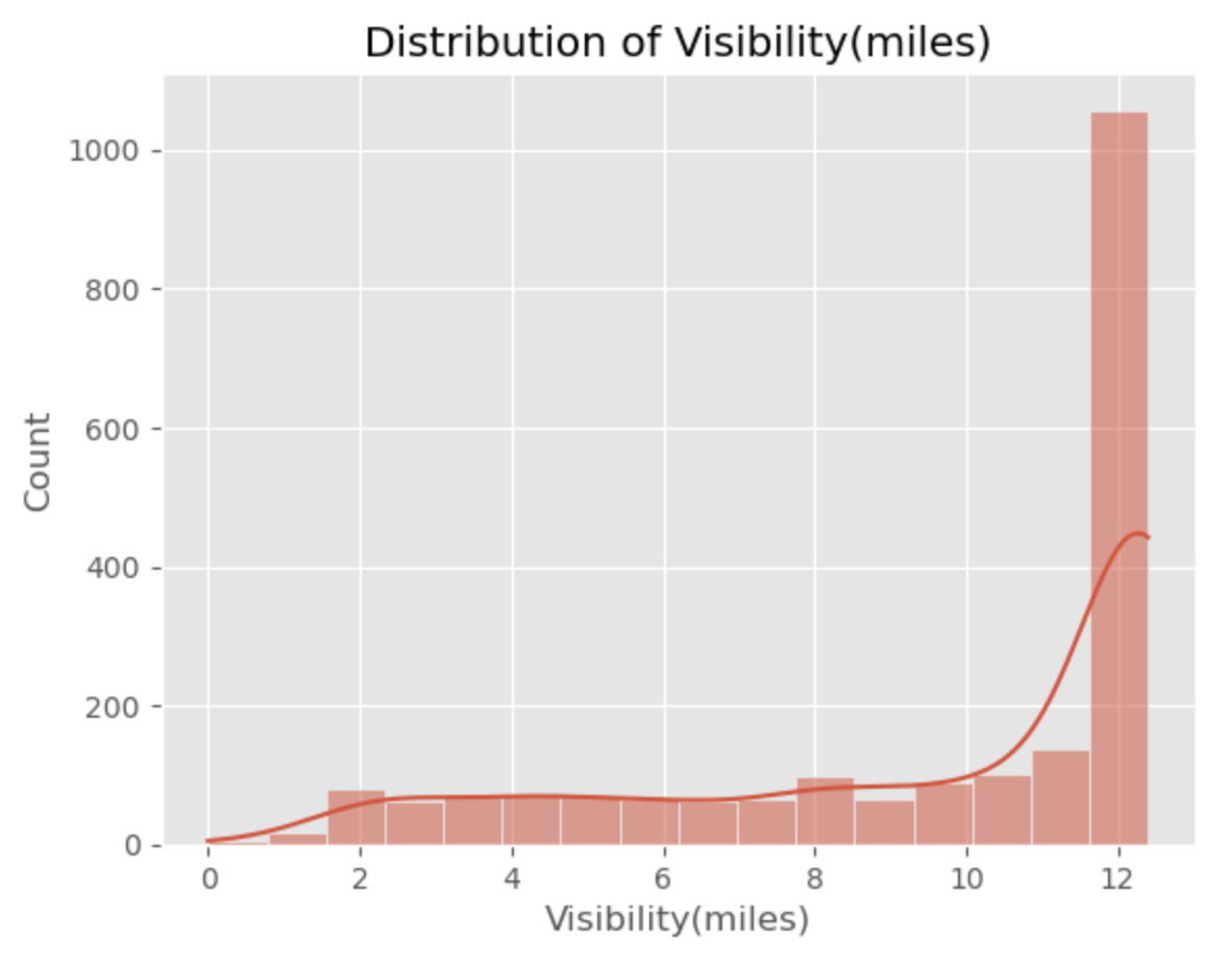
# Missing values of VISIBILITY

# Plotting 'Visibility(miles)'
sns.histplot(x = 'Visibility(miles)',
            data = df_full,
            kde = True)

# Title and labels
plt.title (label  = 'Distribution of Visibility(miles)')
plt.xlabel(xlabel = 'Visibility(miles)')
plt.ylabel(ylabel = 'Count')

# Displaying the plot
plt.show()

Output: linearly separable data

fill1 = df_full['Visibility(miles)'].median()
# Imputing Visibility(miles)
df_full['Visibility(miles)'].fillna(value   = fill1,
                                    inplace = True)

# Check the correct imputation
df_full[ ['Visibility(miles)', 'm_Visibility(miles)'] ][df_full['m_Visibility(miles)'] == 1].head(n = 10)

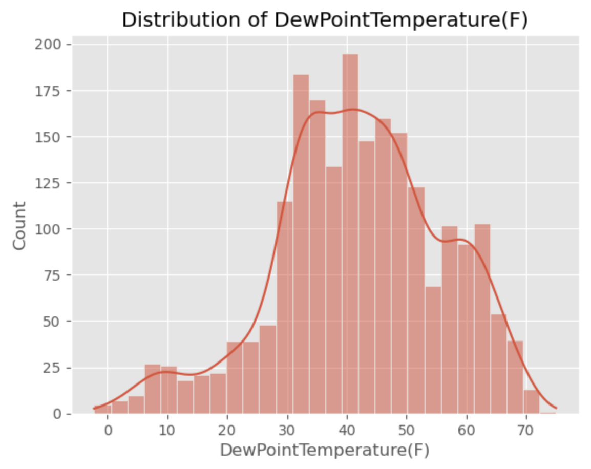
# DewPointTemperature
df_full[['DewPointTemperature(F)' , 'm_Dew

PointTemperature(F)']].describe()

# Plotting 'DewPointTemperature'
sns.histplot(x = 'DewPointTemperature(F)',
            data = df_full,
            kde = True)

# Title and labels
plt.title (label  = 'Distribution of DewPointTemperature(F)')
plt.xlabel(xlabel = 'DewPointTemperature(F)')
plt.ylabel(ylabel = 'Count')

# Displaying the plot
plt.show()

Output: linearly separable data

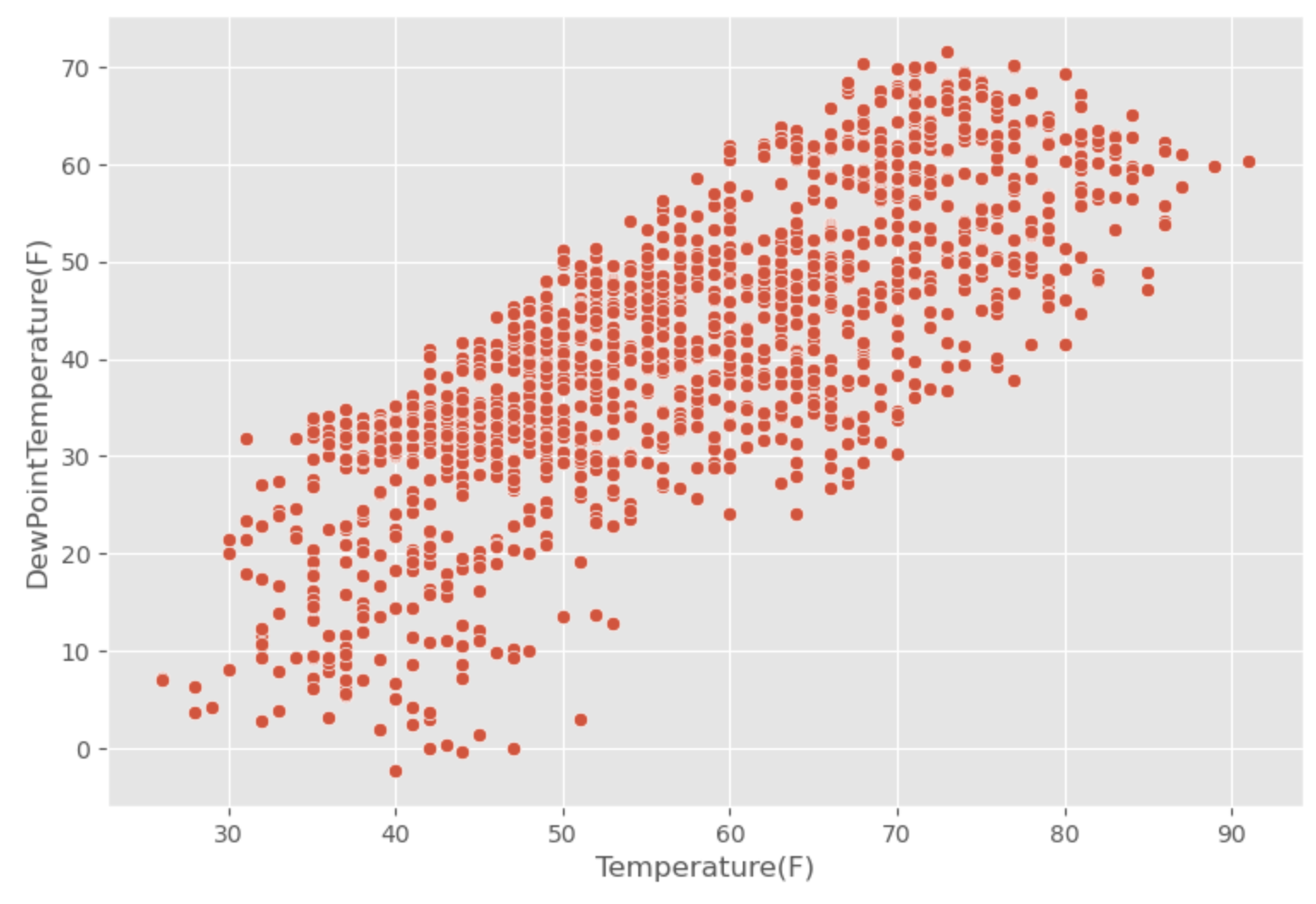
# Setting figure size
fig, ax = plt.subplots(figsize = (9, 6))

# Developing a scatterplot
sns.scatterplot(x    = "Temperature(F)",
         y    = "DewPointTemperature(F)",
         data = data_0)

# Showing the results
plt.show()

Output: linearly separable data

# Converting F to C
df_full['Temperature(C)']=(df_full['Temperature(F)']-32)*5/9

# Using the DewPoint Temperature Formula to estimate the real value in F
fill2=((df_full['Temperature(C)']-((100-df_full['Humidity(%)'])/5))*9/5)+32

# Imputing missing values
df_full['DewPointTemperature(F)'].fillna(value=fill2,
                          inplace = True)
# Delete the new column created
df_full.drop(columns=['Temperature(C)'], inplace=True)

# Check the correct imputation
df_full[ ['DewPointTemperature(F)', 'm_DewPointTemperature(F)','Temperature(F)','Humidity(%)'] ][df_full['m_DewPointTemperature(F)'] == 1].head(n = 10)

# Plotting 'SolarRadiation(MJ/m2)'
sns.histplot(x = 'SolarRadiation(MJ/m2)',
            data = df_full,
            kde = True)

# Title and labels
plt.title (label  = 'Distribution of SolarRadiation(MJ/m2)')
plt.xlabel(xlabel = 'SolarRadiation(MJ/m2)')
plt.ylabel(ylabel = 'Count')

# Displaying the plot
plt.show()

Output: linearly separable data

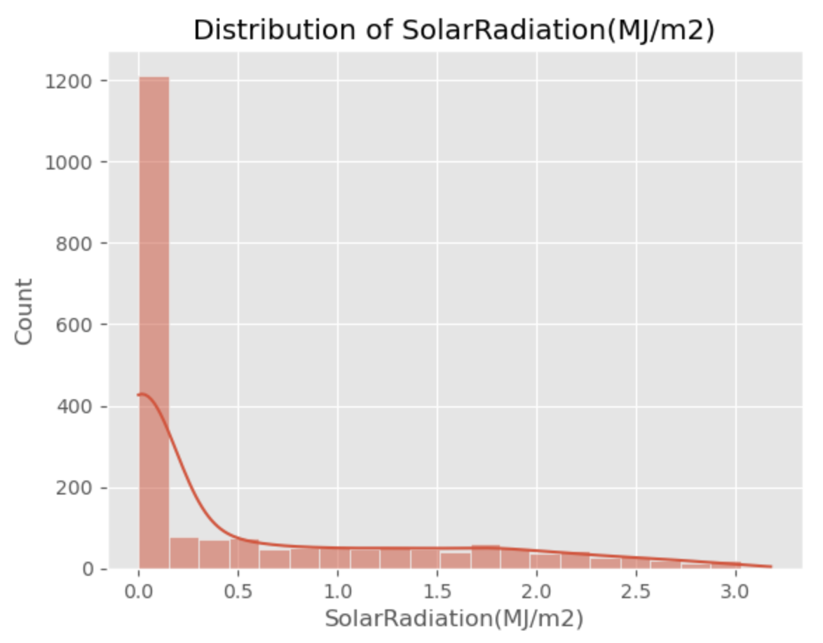
# Imputing SolarRadiation(MJ/m2)
df_full['SolarRadiation(MJ/m2)'].fillna(value   = 0   ,
                               inplace = True)

df_full[ ['SolarRadiation(MJ/m2)', 'm_SolarRadiation(MJ/m2)'] ][df_full['m_SolarRadiation(MJ/m2)'] == 1].head(n = 10)

# Making sure all missing values have been taken care of
df_full.isnull().sum(axis = 0)

# Scatterplot AFTER missing values
sns.histplot(data  = df_full,
             x     = 'Visibility(miles)',
             fill  = True,
             color = "red")

# Scatterplot BEFORE missing values
sns.histplot(data  = df_full_mv,
             x     = 'Visibility(miles)',
             fill  = True,
             color = 'black')

# Mean lines
plt.axvline(df_full['Visibility(miles)'].mean()   , color = "red")
plt.axvline(df_full_mv['Visibility(miles)'].mean(), color = "blue")

# Labels and rendering
plt.title (label  = "Imputation Results (Visibility(miles))")
plt.xlabel(xlabel = "Visibility(miles)")
plt.ylabel(ylabel = "Frequency")
plt.show()

# Scatterplot AFTER missing values
sns.histplot(data  = df_full,
             x     = 'DewPointTemperature(F)',
             fill  = True,
             color = "red")

# Scatterplot BEFORE missing values
sns.histplot(data  = df_full_mv,
             x     = 'DewPointTemperature(F)',
             fill  = True,
             color = 'black')

# Mean lines
plt.axvline(df_full['DewPointTemperature(F)'].mean()   , color = "red")
plt.axvline(df_full_mv['DewPointTemperature(F)'].mean(), color = "blue")

# Labels and rendering
plt.title (label  = "Imputation Results (DewPointTemperature(F))")
plt.xlabel(xlabel = "DewPointTemperature(F)")
plt.ylabel(ylabel = "Frequency")
plt.show()

# Scatterplot AFTER missing values
sns.histplot(data  = df_full,
             x     = 'SolarRadiation(MJ/m2)',
             fill  = True,
             color = "red")

# Scatterplot BEFORE missing values
sns.histplot(data  = df_full_mv,
             x     = 'SolarRadiation(MJ/m2)',
             fill  = True,
             color = 'black')

# Mean lines
plt.axvline(df_full['SolarRadiation(MJ/m2)'].mean()   , color = "red")
plt.axvline(df_full_mv['SolarRadiation(MJ/m2)'].mean(), color = "blue")

# Labels and rendering
plt.title (label  = "Imputation Results (SolarRadiation(MJ/m2))")
plt.xlabel(xlabel = "SolarRadiation(MJ/m2)")
plt.ylabel(ylabel = "Frequency")
plt.show()

Exploratory Data Analysis and Data Preprocessing

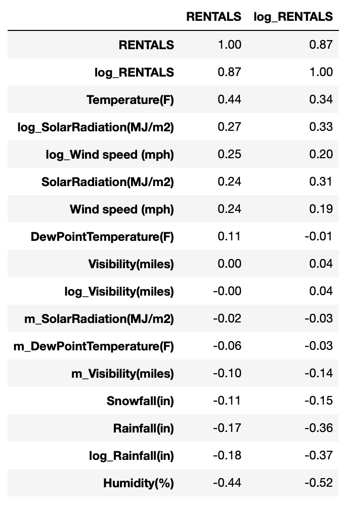
The exploratory data analysis commenced with a review of descriptive statistics, uncovering a wide range of rental counts and diverse weather conditions. Histograms of rental counts illustrated a right-skewed distribution, suggesting variability in daily usage patterns. Correlation analysis highlighted potential predictors, such as temperature and humidity, albeit with varying degrees of association. Notably, the presence of missing values in visibility, dew point temperature, and solar radiation necessitated thoughtful imputation strategies. The preprocessing phase also addressed categorical variables through one-hot encoding, ensuring compatibility with machine learning algorithms. Standardization of continuous variables was paramount to eliminate scale discrepancies, thereby facilitating more balanced contributions across features.

Transformations

# Transformations

# Developing a histogram using HISTPLOT
sns.histplot(data   = df_full[df_full['FunctioningDay']=='Yes'],
             x      = 'RENTALS',
             kde    = True)

# Title and axis labels
plt.title(label   = "Original Distribution of RENTALS")
plt.xlabel(xlabel = "RENTALS") # avoiding using dataset labels
plt.ylabel(ylabel = "Count")

# Displaying the histogram
plt.show()

# Log transforming Sale_Price and saving it to the dataset
df_full['log_RENTALS'] = np.log1p(df_full['RENTALS'])

# Developing a histogram using HISTPLOT
sns.histplot(data   = df_full[df_full['FunctioningDay']=='Yes'],
             x      = 'log_RENTALS',
             kde    = True)

# Title and axis labels
plt.title(label   = "Logarithmic Distribution of RENTALS")
plt.xlabel(xlabel = "RENTALS (log)") # avoiding using dataset labels
plt.ylabel(ylabel = "Count")

# Displaying the histogram
plt.show()

df_full.skew(axis = 0, numeric_only = True).round(decimals = 2)

df_full[df_full['FunctioningDay']=='Yes'].skew(axis = 0, numeric_only = True).round(decimals = 2)

# Logarithmically transform any X-features that have an absolute skewness value greater than 1.0.

df_full['log_Wind speed (mph)'] = np.log1p(df_full['Wind speed (mph)'])
df_full['log_Visibility(miles)'] = np.log1p(df_full['Visibility(miles)'])
df_full['log_Rainfall(in)'] = np.log1p(df_full['Rainfall(in)'])
df_full['log_SolarRadiation(MJ/m2)'] = np.log1p(df_full['SolarRadiation(MJ/m2)'])

# Skewness AFTER logarithmic transformations
df_full.loc[ : , 'log_RENTALS': ].skew(axis = 0).round(decimals = 2).sort_index(ascending = False)

# Analyzing (Pearson) correlations
df_corr = df_full[df_full['FunctioningDay']=='Yes'].corr(method = 'pearson',numeric_only = True ).round(2)

df_corr.loc[ : , ['RENTALS', 'log_RENTALS'] ].sort_values(by = 'RENTALS',
                                                                ascending = False)

Output: linearly separable data

Feature Engineering

# Feature Engineering
# Counting the number of zeroes for 
windspeed_zeroes  = len(df_full['Wind speed (mph)'][df_full['Wind speed (mph)']==0]) 
visibility_zeroes   = len(df_full['Visibility(miles)'][df_full['Visibility(miles)']==0]) 
dwpt_zeroes     = len(df_full['DewPointTemperature(F)'][df_full['DewPointTemperature(F)']==0]) 
rainfall_zeroes = len(df_full['Rainfall(in)'][df_full['Rainfall(in)']==0]) 
snowfall_zeroes    = len(df_full['Snowfall(in)'][df_full['Snowfall(in)']==0]) 
solar_zeroes  = len(df_full['SolarRadiation(MJ/m2)'][df_full['SolarRadiation(MJ/m2)']==0]) 

# Printing a table of the results
print(f"""
                 No\t\tYes
               ---------------------
WindSpeed     | {windspeed_zeroes}\t\t{len(df_full) - windspeed_zeroes}
Visibility    | {visibility_zeroes}\t\t{len(df_full) - visibility_zeroes}
DewPoint      | {dwpt_zeroes}\t\t{len(df_full) - dwpt_zeroes}
Rainfall      | {rainfall_zeroes}\t\t{len(df_full) - rainfall_zeroes}
Snowfall      | {snowfall_zeroes}\t\t{len(df_full) - snowfall_zeroes}
SolarRadiatio | {solar_zeroes}\t\t{len(df_full

) - solar_zeroes}
""")

# Placeholder variables
df_full['has_SolarRadiation'] = 0

# Iterating over each original column to change values in the new feature columns
for index, value in df_full.iterrows():
    if df_full.loc[index, 'SolarRadiation(MJ/m2)'] > 0:
        df_full.loc[index, 'has_SolarRadiation'] = 1

# Checking results
df_full[  ['has_SolarRadiation']  ].head(n = 5)

# Developing a small correlation matrix
new_corr = df_full[df_full['FunctioningDay']=='Yes'].corr(method = 'pearson', numeric_only = True).round(decimals = 2)

# Checking the correlations of the newly-created variables with Sale_Price
new_corr.loc[ ['has_SolarRadiation'],
              ['RENTALS', 'log_RENTALS'] ].sort_values(by = 'RENTALS',
                                                             ascending = False)

# CATEGORICAL DATA

# Printing columns
print(f"""
Holiday
------
{df_full['Holiday'].value_counts()}

FunctioningDay
----------
{df_full['FunctioningDay'].value_counts()}
""")

# Defining a function for categorical boxplots
def categorical_boxplots(response, cat_var, data):
    """
	This function is designed to generate a boxplot for  can be used for categorical variables.
    Make sure matplotlib.pyplot and seaborn have been imported (as plt and sns).

    PARAMETERS
	----------
	response : str, response variable
	cat_var  : str, categorical variable
	data     : DataFrame of the response and categorical variables
	"""

    fig, ax = plt.subplots(figsize = (10, 8))
    
    sns.boxplot(x    = response,
                y    = cat_var,
                data = data)
    
    plt.suptitle("")
    plt.show()

# Calling the function for Holiday
categorical_boxplots(response = 'RENTALS',
					 cat_var  = 'Holiday',
					 data     = df_full)

# Calling the function for FunctioningDay
categorical_boxplots(response = 'RENTALS',
					 cat_var  = 'FunctioningDay',
					 data     = df_full)

# One hot encoding categorical variables
one_hot_Holiday = pd.get_dummies(df_full['Holiday'], prefix = 'Holiday')
one_hot_FunctioningDay = pd.get_dummies(df_full['FunctioningDay'], prefix = 'FunctioningDay')

# Dropping categorical variables after they've been encoded
df_full = df_full.drop('Holiday', axis = 1)
df_full = df_full.drop('FunctioningDay', axis = 1)

# Joining codings together
df_full = df_full.join([one_hot_Holiday,one_hot_FunctioningDay ])

# Saving new columns
new_columns = df_full.columns

# Checking results
df_full.head(n = 5)

# Creating a (Pearson) correlation matrix
df_corr = df_full[(df_full['FunctioningDay_Yes'] == True) & (df_full['set'] == 'Not Kaggle')].corr(numeric_only = True).round(2)

# Printing (Pearson) correlations with SalePrice
df_corr.loc[ : , ['RENTALS', 'log_RENTALS'] ].sort_values(by = 'RENTALS',
                                                                ascending = False)

# Converting DataHour in datetime type
df_full['DateHour'] = pd.to_datetime(df_full['DateHour'])

# Get the year, month, day, hour, and week day
df_full['Year'] = df_full['DateHour'].dt.year
df_full['Month'] = df_full['DateHour'].dt.month
df_full['Day'] = df_full['DateHour'].dt.day
df_full['Hour'] = df_full['DateHour'].dt.hour
df_full['DayOfWeek'] = df_full['DateHour'].dt.weekday

# Checking new columns
df_full[['DateHour', 'Year', 'Month', 'Day', 'Hour', 'DayOfWeek']].head()

df_full[['DateHour', 'Year', 'Month', 'Day', 'Hour', 'DayOfWeek']].describe()

df_full['Day_Month'] = df_full['Day'].astype(str).str.zfill(2) + '-' + df_full['Month'].astype(str).str.zfill(2)

sns.lineplot(data = df_full[df_full['FunctioningDay_Yes'] == True],
            x = 'Day_Month',
            y ='RENTALS')

# Title and axis labels
plt.title(label   = "Distribution of RENTALS")
plt.xlabel(xlabel = "RENTALS") # avoiding using dataset labels
plt.ylabel(ylabel = "Count")

# Displaying the histogram
plt.show()

# Converting day of week into rad 
df_full['DayOfWeek_rad'] = (2 * np.pi * df_full['DayOfWeek']) / 7

# Creating cycle variables for each day of week 
df_full['DayOfWeek_sin'] = np.sin(df_full['DayOfWeek_rad'])
df_full['DayOfWeek_cos'] = np.cos(df_full['DayOfWeek_rad'])

df_full = pd.get_dummies(df_full, columns=['DayOfWeek'], prefix='weekday', drop_first=True)

# New feature: One of the most well-known formulas for calculating the heat index is the Steadman formula.
df_full['heatIndex'] = 0.5*(df_full['Temperature(F)'] + 61.0 + ((df_full['Temperature(F)']-68.0)*1.2)+(df_full['Humidity(%)']*0.094))

# New feature indicating poor weather conditions based on visibility, rainfall, and snowfall

# Define thresholds
visibility_threshold = 7  
rainfall_threshold = 0.1

# Create 'PoorWeather' column based on the defined criteria
df_full['PoorWeather'] = ((df_full['Visibility(miles)'] <= visibility_threshold) |
                          (df_full['Rainfall(in)'] > rainfall_threshold) |
                          (df_full['Snowfall(in)'] > 0)).astype(int)

# Creating a (Pearson) correlation matrix
df_corr = df_full[(df_full['FunctioningDay_Yes'] == True) & (df_full['set'] == 'Not Kaggle')].corr(numeric_only = True).round(2)

# Printing (Pearson) correlations with SalePrice
df_corr.loc[ : , ['RENTALS', 'log_RENTALS'] ].sort_values(by = 'RENTALS',
                                                                ascending = False)

df_full = df_full.drop(columns=['DateHour', 'Year','Day_Month'])

# Subsetting for RENTALS
rental_corr = df_corr.loc[ : , ['RENTALS', 'log_RENTALS'] ].sort_values(by = 'RENTALS',
                                                                 ascending = False)
# Removing irrelevant correlations
rental_corr = rental_corr.iloc[ 2: , : ]

# Placeholder column for y-variable recommendation
rental_corr['original_v_log'] = 0

# Filling in placeholder
for index, column in rental_corr.iterrows():
    if abs(rental_corr.loc[ index, 'RENTALS']) >  abs(rental_corr.loc[ index, 'log_RENTALS']):
        rental_corr.loc[ index , 'original_v_log'] = 'RENTALS'
    elif abs(rental_corr.loc[ index, 'RENTALS']) <  abs(rental_corr.loc[ index, 'log_RENTALS']):
        rental_corr.loc[ index , 'original_v_log'] = 'log_RENTALS'
    else:
        rental_corr.loc[ index , 'original_v_log'] = 'Tie'

# Checking results
rental_corr["original_v_log"].value_counts(normalize = False,
                                       sort      = True,
                                       ascending = False).round(decimals = 2)

df_full.head()

Standardization

# Standardization

# Preparing explanatory variable data
df_full_data   = df_full.drop(['RENTALS',
                               'log_RENTALS',
                                'set','FunctioningDay_No','FunctioningDay_Yes'],
                                axis = 1)

# Preparing the target variable
df_full_target = df_full.loc[ : , ['RENTALS',
                               'log_RENTALS',
                                   'set','FunctioningDay_No','FunctioningDay_Yes']]

# Instantiating a StandardScaler() object
scaler = StandardScaler()

# Fitting the scaler with the data
scaler.fit(df_full_data)

# Transforming our data after fit
x_scaled = scaler.transform(df_full_data)

# Converting scaled data into a DataFrame
x_scaled_df = pd.DataFrame(x_scaled)

# Checking the results
x_scaled_df.describe(include = 'number').round(decimals = 2)

# Adding labels to the scaled DataFrame
x_scaled_df.columns = df_full_data.columns

# Checking pre- and post-scaling of the data
print(f"""
Dataset BEFORE Scaling
----------------------
{np.var(df_full_data)}

Dataset AFTER Scaling
----------------------
{np.var(x_scaled_df)}
""")

x_scaled_df.info()

df_full_target.info()

x_scaled_df.index = df_full_target.index

df_full = pd.concat([x_scaled_df, df_full_target], axis=1)

df_full = df_full.rename(columns={
    'Temperature(F)': 'Temperature_F',
    'Humidity(%)': 'Humidity',
    'Wind speed (mph)': 'Wind_speed',
    'Visibility(miles)': 'Visibility',
    'DewPointTemperature(F)': 'DewPointTemperature',
    'Rainfall(in)': 'Rainfall',
    'Snowfall(in)': 'Snowfall',
    'SolarRadiation(MJ/m2)': 'SolarRadiation',
    'm_Visibility(miles)': 'm

_Visibility',
    'm_DewPointTemperature(F)': 'm_m_DewPointTemperature',
    'm_SolarRadiation(MJ/m2)': 'm_SolarRadiation',
    'log_Wind speed (mph)': 'log_Wind_speed',
    'log_Visibility(miles)': 'log_Visibility',
    'log_Rainfall(in)': 'log_Rainfall',
    'log_SolarRadiation(MJ/m2)': 'log_SolarRadiation'
})

df_train_1 = df_full[ (df_full['set'] == 'Not Kaggle') & (df_full['FunctioningDay_Yes'] == True)]

# Making a copy of housing
df_full_explanatory = df_full[ df_full['set'] == 'Not Kaggle' ].copy()

# Dropping SalePrice and Order from the explanatory variable set
df_full_explanatory = df_full_explanatory.drop([
                                 'RENTALS',
                                 'log_RENTALS',
                                 'set'], axis = 1)

# Formatting each explanatory variable for statsmodels
for val in df_full_explanatory:
    print(val,"+")

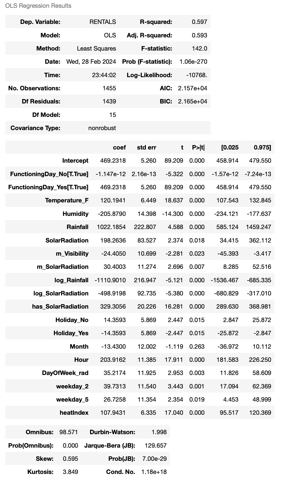
# Building a full model

# Blueprinting a model type
lm_full = smf.ols(formula = """RENTALS ~ Temperature_F +
Humidity +
Rainfall +
SolarRadiation +
m_Visibility +
m_SolarRadiation +
log_Rainfall +
log_SolarRadiation +
has_SolarRadiation +
Holiday_No +
Holiday_Yes +
FunctioningDay_No +
FunctioningDay_Yes +
Month +
Hour +
DayOfWeek_rad +
weekday_2 +
weekday_5 +
heatIndex """,
                               data = df_train_1)

# Telling Python to run the data through the blueprint
results_full = lm_full.fit()

# Printing the results
results_full.summary()

Output: linearly separable data

Part III: Data Partitioning

Separating the Kaggle Data

# Parsing out testing data (needed for later)

# Dataset for kaggle
kaggle_data = df_full[ df_full['set'] == 'Kaggle' ].copy()

# Dataset for model building
df = df_full[ df_full['set'] == 'Not Kaggle' ].copy()

# Dropping set identifier (kaggle)
kaggle_data.drop(labels = 'set',
                 axis = 1,
                 inplace = True)

# Dropping set identifier (model building)
df.drop(labels = 'set',
        axis = 1,
        inplace = True)

df = df[ df['FunctioningDay_Yes'] == True ].copy()
df.info()

Train-Test Split

# Train-Test Split
# Note that the following code will remove non-numeric features, keeping only integer and float data types. It will also remove any observations that contain missing values. This is to prevent errors in the model building process. 

# Choosing your x-variables
x_features = ['Temperature_F', 
              'Humidity',
              'Visibility', 
              'DewPointTemperature', 
              'Rainfall',
              'log_Wind_speed', 
              'log_SolarRadiation', 
              'has_SolarRadiation',
              'Month', 'Day', 
              'Hour', 
              'heatIndex',
              'RENTALS', ] 
# This should be a list

# Removing non-numeric columns and missing values
df = df[x_features].copy().select_dtypes(include=[int, float]).dropna(axis = 0)

# Prepping data for train-test split
x_data = df.drop(labels = y_variable,
                 axis   = 1)

y_data = df[y_variable]

# Train-test split (to validate the model)
x_train, x_test, y_train, y_test = train_test_split(x_data, 
                                                    y_data, 
                                                    test_size    = 0.25,
                                                    random_state = 702 )

# Results of train-test split
print(f"""
Original Dataset Dimensions
---------------------------
Observations (Rows): {df.shape[0]}
Features  (Columns): {df.shape[1]}

Training Data (X-side)
----------------------
Observations (Rows): {x_train.shape[0]}
Features  (Columns): {x_train.shape[1]}

Training Data (y-side)
----------------------
Feature Name:        {y_train.name}
Observations (Rows): {y_train.shape[0]}

Testing Data (X-side)
---------------------
Observations (Rows): {x_test.shape[0]}
Features  (Columns): {x_test.shape[1]}

Testing Data (y-side)
---------------------
Feature Name:        {y_test.name}
Observations (Rows): {y_test.shape[0]}
""")

Part IV: Candidate Modeling

Model Development

# Candidate Modeling

# Choosing your x-variables
# Naming the model
model_name = "Linear_Regression" # Name your model

# Model type
model = sklearn.linear_model.LinearRegression() # Model type ( ex: sklearn.linear_model.LinearRegression() )

# Fitting to the training data
model_fit = model.fit(x_train, y_train)

# Predicting on new data
model_pred = model.predict(x_test)

# Scoring the results
model_train_score = model.score(x_train, y_train).round(4)
model_test_score  = model.score(x_test, y_test).round(4)
model_gap         = abs(model_train_score - model_test_score).round(4)
    
# Dynamically printing results
model_summary =  f"""\
Model Name:     {model_name}
Train_Score:    {model_train_score}
Test_Score:     {model_test_score}
Train-Test Gap: {model_gap}
"""

print(model_summary)

Model Name: Linear_Regression
Train_Score: 0.5681
Test_Score: 0.5948
Train-Test Gap: 0.0267

# Candidate Modeling

# Choosing your x-variables
# Naming the model
model_name = "KNN" # Name your model

# Model type
model = KNeighborsRegressor(algorithm = 'auto',
                   n_neighbors = 4) # Model type ( ex: sklearn.linear_model.LinearRegression() )

# Fitting to the training data
model_fit = model.fit(x_train, y_train)

# Predicting on new data
model_pred = model.predict(x_test)

# Scoring the results
model_train_score = model.score(x_train, y_train).round(4)
model_test_score  = model.score(x_test, y_test).round(4)
model_gap         = abs(model_train_score - model_test_score).round(4)
    
# Dynamically printing results
model_summary =  f"""\
Model Name:     {model_name}
Train_Score:    {model_train_score}
Test_Score:     {model_test_score}
Train-Test Gap: {model_gap}
"""

print(model_summary)

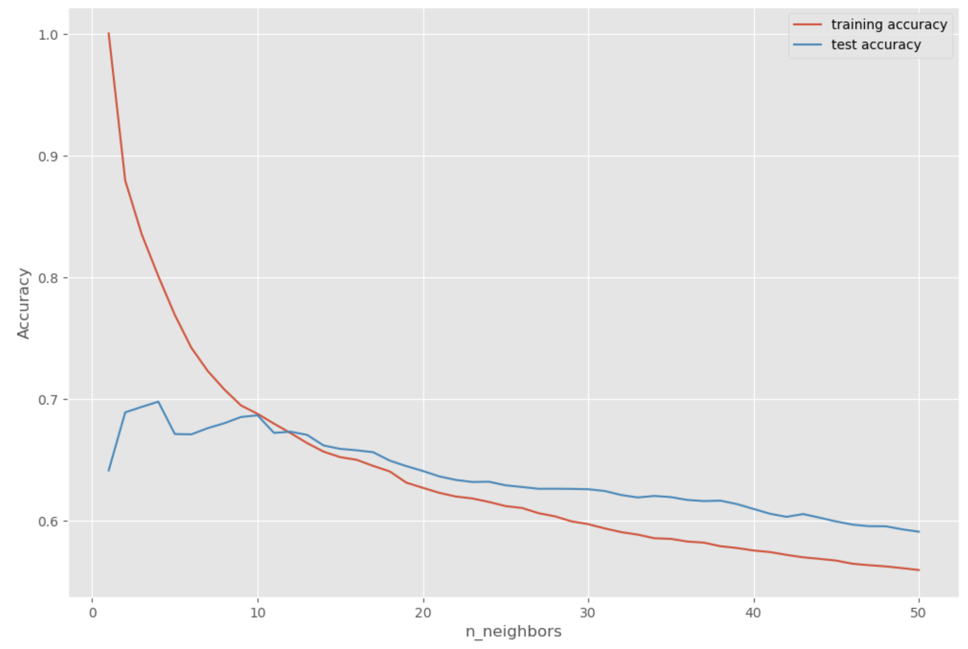
Model Name: KNN
Train_Score: 0.8006
Test_Score: 0.6974
Train-Test Gap: 0.1032

Visualizing KNN Performance

# Creating lists for training set accuracy and test set accuracy
training_accuracy = []
test_accuracy     = []

# Building a visualization of 1 to 50 neighbors
neighbors_settings = range(1, 51)

for n_neighbors in neighbors_settings:
    # Building the model
    clf = KNeighborsRegressor(n_neighbors = n_neighbors)
    clf.fit(x_train, y_train)
    
    # Recording the training set accuracy
    training_accuracy.append(clf.score(x_train, y_train))
    
    # Recording the generalization accuracy
    test_accuracy.append(clf.score(x_test, y_test))

# Plotting the visualization
fig, ax = plt.subplots(figsize=(12,8))
plt.plot(neighbors_settings, training_accuracy, label = "training accuracy")
plt.plot(neighbors_settings, test_accuracy, label = "test accuracy")
plt.ylabel("Accuracy")
plt.xlabel("n_neighbors")
plt.legend()
plt.show()

# Finding the optimal number of neighbors
opt_neighbors = test_accuracy.index(max(test_accuracy)) + 1
print(f"""The optimal number of neighbors is {opt_neighbors}""")

Output: linearly separable data

Further Model Development

# Candidate Modeling

# Choosing your x-variables
# Naming the model
model_name = "Lasso (scaled)" # Name your model

# Model type
model = sklearn.linear_model.Lasso(alpha       = 10.0,
                                  random_state = 702) # Model type ( ex: sklearn.linear_model.LinearRegression() )

# Fitting to the training data
model_fit = model.fit(x_train, y_train)

# Predicting on new data
model_pred = model.predict(x_test)

# Scoring the results
model_train_score = model.score(x_train, y_train).round(4)
model_test_score  = model.score(x_test, y_test).round(4)
model_gap         = abs(model_train_score - model_test_score).round(4)
    
# Dynamically printing results
model_summary =  f"""\
Model Name:     {model_name}
Train_Score:    {model_train_score}
Test_Score:     {model_test_score}
Train-Test Gap: {model_gap}
"""

print(model_summary)

Model Name: Lasso (scaled)
Train_Score: 0.5602
Test_Score: 0.586
Train-Test Gap: 0.0258

# Candidate Modeling

# Choosing your x-variables
# Naming the model
model_name = "Ridge (scaled)" # Name your model

# Model type
model = sklearn.linear_model.Ridge(alpha = 10.0,
                                   random_state = 702) # Model type ( ex: sklearn.linear_model.LinearRegression() )

# Fitting to the training data
model_fit = model.fit(x_train, y_train)

# Predicting on new data
model_pred = model.predict(x_test)

# Scoring the results
model_train_score = model.score(x_train, y_train).round(4)
model_test_score  = model.score(x_test, y_test).round(4)
model_gap         = abs(model_train_score - model_test_score).round(4)
    
# Dynamically printing results
model_summary =  f"""\
Model Name:

     {model_name}
Train_Score:    {model_train_score}
Test_Score:     {model_test_score}
Train-Test Gap: {model_gap}
"""

print(model_summary)

Model Name: Ridge (scaled)
Train_Score: 0.5678
Test_Score: 0.595
Train-Test Gap: 0.0272

# Candidate Modeling

# Choosing your x-variables
# Naming the model
model_name = "Elastic Net (scaled) with MSE" # Name your model

# Model type
model = sklearn.linear_model.SGDRegressor(alpha = 0.5,
                                          penalty = 'elasticnet',
                                         random_state = 702) # Model type ( ex: sklearn.linear_model.LinearRegression() )

# Fitting to the training data
model_fit = model.fit(x_train, y_train)

# Predicting on new data
model_pred = model.predict(x_test)

# Scoring the results
model_train_score = model.score(x_train, y_train).round(4)
model_test_score  = model.score(x_test, y_test).round(4)
model_gap         = abs(model_train_score - model_test_score).round(4)
    
# Dynamically printing results
model_summary =  f"""\
Model Name:     {model_name}
Train_Score:    {model_train_score}
Test_Score:     {model_test_score}
Train-Test Gap: {model_gap}
"""

print(model_summary)

Model Name: Elastic Net (scaled) with MSE
Train_Score: 0.5048
Test_Score: 0.531
Train-Test Gap: 0.0262

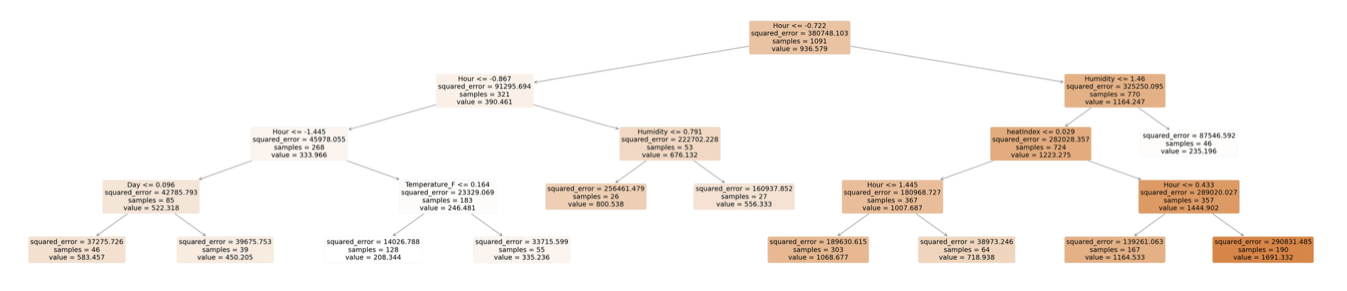
# Candidate Modeling

# Choosing your x-variables
# Naming the model
model_name = "Pruned Regression Tree" # Name your model

# Model type
model = DecisionTreeRegressor(max_depth = 4,
                              min_samples_leaf = 25,
                              random_state = 702) # Model type ( ex: sklearn.linear_model.LinearRegression() )

# Fitting to the training data
model_fit = model.fit(x_train, y_train)

# Predicting on new data
model_pred = model.predict(x_test)

# Scoring the results
model_train_score = model.score(x_train, y_train).round(4)
model_test_score  = model.score(x_test, y_test).round(4)
model_gap         = abs(model_train_score - model_test_score).round(4)
    
# Dynamically printing results
model_summary =  f"""\
Model Name:     {model_name}
Train_Score:    {model_train_score}
Test_Score:     {model_test_score}
Train-Test Gap: {model_gap}
"""

print(model_summary)

# Setting figure size
plt.figure(figsize=(50, 10)) # Adjusting to better fit the visual

# Developing a plotted tree
plot_tree(decision_tree = model, # Changing to pruned_tree_fit
          feature_names = list(x_train.columns),
          filled        = True, 
          rounded       = True, 
          fontsize      = 14)

# Rendering the plot
plt.show()

# Plotting feature importance
def plot_feature_importances(model, train, export = False):
    """
    Plots the importance of features from a CART model.
    
    PARAMETERS
    ----------
    model  : CART model
    train  : explanatory variable training data
    export : whether or not to export as a .png image, default False
    """
    
    # Declaring the number
    n_features = x_train.shape[1]
    
    # Setting plot window
    fig, ax = plt.subplots(figsize=(12,9))
    
    plt.barh(range(n_features), model.feature_importances_, align='center')
    plt.yticks(np.arange(n_features), train.columns)
    plt.xlabel("Feature importance")
    plt.ylabel("Feature")
    
    if export == True:
        plt.savefig('Tree_Leaf_50_Feature_Importance.png')

# Plotting feature importance
plot_feature_importances(model,
                         train = x_train,
                         export = False)

Model Name: Pruned Regression Tree
Train_Score: 0.6138
Test_Score: 0.6222
Train-Test Gap: 0.0084

Output: linearly separable data

Residual Analysis

# Residual Analysis

# Organizing residuals
model_residuals = {"True"            : y_test,
                   "Predicted"       : model_pred
                  }

# Converting residuals into df
model_resid_df = pd.DataFrame(data = model_residuals)

# Checking results
model_resid_df.head(n = 5)

Hyperparameter Tuning

# Hyperparameter Tuning
# Declaring a hyperparameter space
criterion_range = ["squared_error", "friedman_mse", "absolute_error", "poisson"]
splitter_range  = ["best", "random"]
depth_range     = np.arange(1,11,1)
leaf_range      = np.arange(1,251,5)

# Creating a hyperparameter grid
param_grid = {'criterion'      : criterion_range,
             'splitter'        : splitter_range,
             'max_depth'       : depth_range,
             'min_samples_leaf': leaf_range}

# Instantiating the model object without hyperparameters
tuned_tree = DecisionTreeRegressor()

# RandomizedSearchCV object
tuned_tree_cv = RandomizedSearchCV(estimator             = tuned_tree, # Model
                                   param_distributions   = param_grid, # Hyperparameter ranges
                                   cv                    = 5,    # Folds
                                   n_iter                = 1000, # How many models to build
                                   random_state          = 702)

# Fitting to the FULL DATASET (due to cross-validation)
tuned_tree_cv.fit(x_train, y_train)

# Printing the optimal parameters and best score
print("Tuned Parameters  :", tuned_tree_cv.best_params_)
print("Tuned Training AUC:", tuned_tree_cv.best_score_.round(4))

# Naming the model
model_name = 'Tuned Tree'

# Instantiating a logistic regression model with tuned values
model = DecisionTreeRegressor(splitter         = 'random',
                              min_samples_leaf = 6,
                              max_depth        = 9,
                              criterion        = 'squared_error')

# Fitting to the TRAINING data
model.fit(x_train, y_train)

# Predicting based on the testing set
model.predict(x_test)

# Scoring results
model_train_score = model.score(x_train, y_train).round(4)
model_test_score  = model.score(x_test, y_test).round(4)
model_gap         = abs(model_train_score - model_test_score).round(4)

# Displaying results
print('Training Score :', model_train_score)
print('Testing Score  :', model_test_score)
print('Train-Test Gap :', model_gap)

Training Score : 0.7402
Testing Score : 0.6542
Train-Test Gap : 0.086

# Hyperparameter Tuning
# Declaring a hyperparameter space
n_neighbors = np.arange(1, 31)
weights     = ['uniform', 'distance']
algorithm   = ['ball_tree', 'kd_tree', 'brute', 'auto']
leaf_size   = np.arange(1, 50)
p_size      = [1, 2]

# Creating a hyperparameter grid
param_grid = {
            'n_neighbors': n_neighbors, 
            'weights': weights,
            'algorithm': algorithm,
            'leaf_size': leaf_size,  
            'p': p_size 
}

# Instantiating the model object without hyperparameters
tuned_knn = KNeighborsRegressor()

# RandomizedSearchCV object
tuned_knn_cv = RandomizedSearchCV(estimator             = tuned_knn, # Model
                                   param_distributions   = param_grid, # Hyperparameter ranges
                                   cv                    = 5,    # Folds
                                   n_iter                = 1000, # How many models to build
                                   random_state          = 702)

# Fitting to the FULL DATASET (due to cross-validation)
tuned_knn_cv.fit(x_train, y_train)

# Printing the optimal parameters and best score
print("Tuned Parameters  :", tuned_knn_cv.best_params_)
print("Tuned Training AUC:", tuned_knn_cv.best_score_.round(4))

# Naming the model
model_name = 'Tuned KNN'

# Instantiating a logistic regression model with tuned values
model = KNeighborsRegressor(weights = 'distance',
                            p = 1,
                              n_neighbors        = 5,
                              leaf_size        = 4,
                           algorithm = 'kd_tree')

# Fitting to the TRAINING data
model.fit(x_train, y_train)

# Predicting based on the testing set
model.predict(x_test)

# Scoring results
model_train_score = model.score(x_train, y_train).round(4)
model_test_score  = model.score(x_test, y_test).round(4)
model_gap         = abs(model_train_score - model_test_score).round(4)

# Displaying results
print('Training Score :', model_train_score)
print('Testing Score  :', model_test_score)
print('Train-Test Gap :', model_gap)

Training Score : 1.0
Testing Score : 0.7451
Train-Test Gap : 0.2549

# Hyperparameter Tuning
# Declaring a hyperparameter space
alpha = np.logspace(-4, 4, 200)
max_iter     = [1000, 5000, 10000]
selection   = ['cyclic', 'random']

# Creating a hyperparameter grid
param_grid = {
            'alpha': alpha, 
            'max_iter': max_iter,
            'selection': selection,
}

# Instantiating the model object without hyperparameters
tuned_Lasso = sklearn.linear_model.Lasso()

# RandomizedSearchCV object
tuned_Lasso_cv = RandomizedSearchCV(estimator             = tuned_Lasso, # Model
                                   param_distributions   = param_grid, # Hyperparameter ranges
                                   cv                    = 5,    # Folds
                                   n_iter                = 1000, # How many models to build
                                   random_state          = 702)

# Fitting to the FULL DATASET (due to cross-validation)
tuned_Lasso_cv.fit(x_train, y_train)

# Printing the optimal parameters and best score
print("

Tuned Parameters  :", tuned_Lasso_cv.best_params_)
print("Tuned Training AUC:", tuned_Lasso_cv.best_score_.round(4))

# Naming the model
model_name = 'Tuned Lasso'

# Instantiating a logistic regression model with tuned values
model = sklearn.linear_model.Lasso(selection = 'random',
                                  max_iter = 5000,
                                  alpha = 2.64)

# Fitting to the TRAINING data
model.fit(x_train, y_train)

# Predicting based on the testing set
model.predict(x_test)

# Scoring results
model_train_score = model.score(x_train, y_train).round(4)
model_test_score  = model.score(x_test, y_test).round(4)
model_gap         = abs(model_train_score - model_test_score).round(4)

# Displaying results
print('Training Score :', model_train_score)
print('Testing Score  :', model_test_score)
print('Train-Test Gap :', model_gap)

# Hyperparameter Tuning
# Declaring a hyperparameter space
alpha = np.logspace(-6, 6, 200)
solver     = ['svd', 'cholesky', 'lsqr', 'sag', 'saga']
max_iter   = [None, 1000, 5000, 10000]

# Creating a hyperparameter grid
param_grid = {
            'alpha': alpha, 
            'solver': solver,
            'max_iter': max_iter,
}

# Instantiating the model object without hyperparameters
tuned_Ridge = sklearn.linear_model.Ridge()

# RandomizedSearchCV object
tuned_Ridge_cv = RandomizedSearchCV(estimator             = tuned_Ridge, # Model
                                   param_distributions   = param_grid, # Hyperparameter ranges
                                   cv                    = 5,    # Folds
                                   n_iter                = 1000, # How many models to build
                                   random_state          = 702)

# Fitting to the FULL DATASET (due to cross-validation)
tuned_Ridge_cv.fit(x_train, y_train)

# Printing the optimal parameters and best score
print("Tuned Parameters  :", tuned_Ridge_cv.best_params_)
print("Tuned Training AUC:", tuned_Ridge_cv.best_score_.round(4))

# Naming the model
model_name = 'Tuned Ridge'

# Instantiating a logistic regression model with tuned values
model = sklearn.linear_model.Ridge(solver = 'cholesky',
                                  max_iter = 1000,
                                  alpha = 8.603464416684492)

# Fitting to the TRAINING data
model.fit(x_train, y_train)

# Predicting based on the testing set
model.predict(x_test)

# Scoring results
model_train_score = model.score(x_train, y_train).round(4)
model_test_score  = model.score(x_test, y_test).round(4)
model_gap         = abs(model_train_score - model_test_score).round(4)

# Displaying results
print('Training Score :', model_train_score)
print('Testing Score  :', model_test_score)
print('Train-Test Gap :', model_gap)

Training Score : 0.5679
Testing Score : 0.5951
Train-Test Gap : 0.0272

Part V: Preparing Submission File for Kaggle

Storing Predicted Values

# Preparing Submission File for Kaggle

# Removing non-numeric columns and missing values
kaggle_df = kaggle_data[x_features].copy()

# x-data
x_data_kaggle = kaggle_df.drop(labels = y_variable,
                               axis   = 1)

# y-data
y_data_kaggle = kaggle_df[y_variable]

# Fitting model from above to the Kaggle test data
kaggle_predictions = model.predict(x_data_kaggle)

# Organizing predictions
model_predictions = {"RENTALS" : kaggle_predictions}

# Converting predictions into df
model_pred_df = pd.DataFrame(data  = model_predictions,
                             index = df_test.index)

model_pred_df.head()

# Reading testing data into Python
testing_data = './datasets/test.xlsx'

# Calling this df_test
df_test_2 = pd.read_excel(io         = testing_data,
                        sheet_name = 'data',
                        header     = 0,
                        index_col  = 'ID')
df_test_2.head()

model_pred_df['FunctioningDay'] = df_test_2['FunctioningDay'].values
model_pred_df.head()

model_pred_df.loc[model_pred_df['FunctioningDay'] == 'No', 'RENTALS'] = 0
model_pred_df.head()

model_pred_df = model_pred_df.drop('FunctioningDay', axis=1)
model_pred_df.head()

# Naming the .csv file
# Sending predictions to .csv
model_pred_df.to_csv(path_or_buf = "./model_output/Solis_Jorge_A1_v3.csv",
                     index       = True,
                     index_label = 'ID')

Conclusion

The comprehensive analysis undertaken in this project involved several key stages: data preprocessing, exploratory data analysis, feature engineering, model development, and hyperparameter tuning. By meticulously cleaning and transforming the dataset, we ensured that the input to our machine learning models was of high quality. The exploratory data analysis provided crucial insights into the relationships and patterns within the data, guiding our feature engineering process to create meaningful and impactful predictors.

We evaluated multiple models, including Linear Regression, Lasso, Ridge, Elastic Net, K-Nearest Neighbors, and Decision Tree Regressor, to predict bike rentals. Each model was assessed based on its performance metrics, such as R-squared values, to ensure the selection of the best-performing model. Hyperparameter tuning further refined the models, optimizing their configurations to achieve the highest predictive accuracy.

The final models demonstrated strong predictive capabilities, with the tuned models showing significant improvement over the base models. The Decision Tree Regressor, in particular, provided valuable insights into feature importance, highlighting the most influential factors affecting bike rentals.

In conclusion, this project successfully developed robust predictive models for forecasting bike rentals, leveraging a variety of machine learning techniques and thorough data preprocessing. The insights gained from this analysis can aid in strategic planning and operational decision-making in the bike-sharing industry, ultimately enhancing efficiency and user satisfaction.

Share on

Twitter Facebook Google+ LinkedIn

Jorge Solis

Predicting Bike Rentals in Chicago Using Machine Learning

Bike Rental Demand Forecasting Project

Introduction

Objective

Part I: Imports and Data Check

Importing Libraries

Importing Data

Concatenating Datasets

Setting Response Variable

Part II: Data Preparation

Base Modeling

Missing Value Analysis and Imputation

Exploratory Data Analysis and Data Preprocessing

Transformations

Feature Engineering

Standardization

Part III: Data Partitioning

Separating the Kaggle Data

Train-Test Split

Part IV: Candidate Modeling

Model Development

Visualizing KNN Performance

Further Model Development

Residual Analysis

Hyperparameter Tuning

Part V: Preparing Submission File for Kaggle

Storing Predicted Values

Conclusion

Share on

You May Also Enjoy

Real Case: Spam Detection Model for Fintech

EY Data Challenge: Coastal Infrastructure Damage Detection using Computer Vision

Case Study: Predicting Clicks in Digital Marketing Campaigns for Air France Airlines

Business Analysis Project: Are Wedding Providers with Sustainable Practices More Cost Effective?