
Case Study: Predicting Clicks in Digital Marketing Campaigns for Air France Airlines
Predicting Clicks in Digital Marketing Campaigns for Air France Airlines
By: Jorge Solis, Initha Paul, Sofia Sorto, Harrison Owusu
Hult International Business School
Jupyter notebook and dataset for this analysis can be found here: Portfolio
Introduction
Air France Airlines conducts various digital marketing campaigns to drive traffic to their website and ultimately increase bookings. The goal of this project is to develop a predictive model to forecast the number of clicks on these campaigns, thereby optimizing future campaign performance.
The business question is: How can we accurately predict the number of clicks for digital marketing campaigns to optimize Air France’s advertising spend?
Business Case from Kellogg School of Management.
Methodology
The project is divided into two parts:
- Data Analysis in R: Analyzing the dataset to preprocess and transform it into a final dataset suitable for modeling.
- Model Development in Python: Using machine learning techniques to predict the number of clicks based on the processed data.
Part I: Data Analysis in R
1. Introduction
The online ticket-selling strategies employed by Air France have proven to be effective in augmenting the number of visits to their website. Media Contacts play a pivotal role in achieving this outcome. As competition intensifies and prices escalate, Media Contacts must leverage their expertise in marketing data analysis to optimize Air France’s returns on investments. A thorough data-driven analysis, complemented by visualizations, was conducted to discern the strengths and weaknesses of the campaign results, thereby enabling the Marketing and Financial teams to make informed decisions on the utilization of the insights and recommendations provided.
Numerical outputs and visualizations were developed, adhering to the principle that “Without this visual analytics solution, one would be stuck analyzing enormous amounts of data in spreadsheets. Instead, the dashboards provide clear actionable insights that drive the business forward.” (Lay)The focus was predominantly on the financial ramifications of the strategies. To this end, outputs were generated, such as the Return on Investment (ROI), which facilitated the understanding and visualization of the profitability of each investment by comparing the gain or loss to its cost and assessing the return on investments. (Beattie, 2024)Additionally, an output that depicted the Conversion Rate between clicks and bookings was devised, accompanied by a respective Bar Chart, to enhance comprehension of each search engine’s performance.
Search Engine Marketing (SEM) inherently involves bidding on keywords pertinent to the advertised business, thereby rendering keyword research a vital component for targeting the desired audience. (Ooi, 2023) By identifying keywords relevant to their business, companies can craft effective ads that will appear when users search for those keywords. Consequently, a focus was placed on word performance, analyzing thedifferent match types of word categories that resulted in bookings.
2. Data Cleaning and Transformation
Here, we handle missing values, remove unnecessary characters, and convert data types to ensure the dataset is clean and ready for analysis.
R Code
#### Setting up the environment

# Install and load necessary packages
install.packages("tidytext",repos = 'http://cran.us.r-project.org' )
install.packages("stringr",repos = 'http://cran.us.r-project.org' )
install.packages("syuzhet",repos = 'http://cran.us.r-project.org')
install.packages("textdata",repos = 'http://cran.us.r-project.org' )
install.packages("DT", repos = 'http://cran.us.r-project.org')
library(dplyr)
library(ggplot2)
library(wordcloud2)
library(tidyverse)
library(tm)
library(tidytext)
library(stringr)
library(syuzhet)
library(textdata)
library(DT)

# Setting up the current working directory
getwd()
setwd("/Users/jorgeluissolis/Documents/0. MAESTRIA HULT/2. SECOND SEMESTER/5. Business Challange II")
getwd()

# Reading the CSV file
data <- read.csv("case_data.csv")

# Display first few rows
head(data, 4)

# Display the structure of the data
str(data, 4)

# Removing dollar sign from the variables
data$Search.Engine.Bid <- gsub("\\$","",data$Search.Engine.Bid)
data$Click.Charges <- gsub("\\$", "",data$Click.Charges)
data$Avg..Cost.per.Click <- gsub("\\$","",data$Avg..Cost.per.Click)
data$Total.Cost..Trans. <- gsub("\\$","",data$Total.Cost..Trans.)
data$Amount <- gsub("\\$","",data$Amount)
data$Total.Cost <- gsub("\\$","",data$Total.Cost)

# Removing percentage sign from the variables
data$Engine.Click.Thru.. <- gsub("\\%","",data$Engine.Click.Thru..)
data$Trans..Conv... <- gsub("\\%","",data$Trans..Conv...)

# Removing commas from the variables
data$Clicks <- gsub(",", "",data$Clicks)
data$Click.Charges <- gsub(",", "",data$Click.Charges)
data$Impressions <- gsub(",","",data$Impressions)
data$Total.Cost..Trans. <- gsub(",","",data$Total.Cost..Trans.)
data$Amount <- gsub(",","",data$Amount)
data$Total.Cost <- gsub(",","",data$Total.Cost)

# Checking for the missing values if any in the data
sum(is.na(data))

# Checking for the incomplete cases in the data
data[!complete.cases(data),]

# Changing datatype from character to numeric
data$Search.Engine.Bid <- as.numeric(data$Search.Engine.Bid)
data$Clicks <- as.numeric(data$Clicks)
data$Click.Charges <- as.numeric(data$Click.Charges)
data$Avg..Cost.per.Click <- as.numeric(data$Avg..Cost.per.Click)
data$Impressions <- as.numeric(data$Impressions)
data$Engine.Click.Thru.. <- as.numeric(data$Engine.Click.Thru..)
data$Trans..Conv... <- as.numeric(data$Trans..Conv...)
data$Total.Cost..Trans. <- as.numeric(data$Total.Cost..Trans.)
data$Amount <- as.numeric(data$Amount)
data$Total.Cost <- as.numeric(data$Total.Cost)
data$Total.Volume.of.Bookings <- as.numeric(data$Total.Volume.of.Bookings)

str(data, 4)

# Checking null values
sum(is.na(data))

# Output 1: Replace the blanks values in Bid Strategy as "NO BID"
data[data$Bid.Strategy == "", "Bid.Strategy"] <- "NO BID"
data[data$Bid.Strategy == "", "Bid.Strategy"]
head(data$Bid.Strategy, 4)

# Output 2: Replace the NA values in match type as "NOT SPECIFIED"
data[data$Match.Type == "N/A", "Match.Type"] <- "Not Specified"
data[data$Match.Type == "N/A", "Match.Type"]
head(data$Match.Type, 4)

# Output 3: Summary statistics of numeric fields
data_statistics <- summary(select(data, where(is.numeric)))
print(head(data_statistics, 5))
3. Exploratory Data Analysis (EDA)
In this section, we visualize and analyze the data to uncover patterns and insights that will guide our feature engineering and model development.
R Code
# Visualization 1: Creating box plots for Publisher and their Average cost for each clicks
publisher_avg_cost <- ggplot(data = data, aes(x = Publisher.Name, y = Avg..Cost.per.Click))
publisher_avg_cost + geom_boxplot()
Output:
Visualization 1
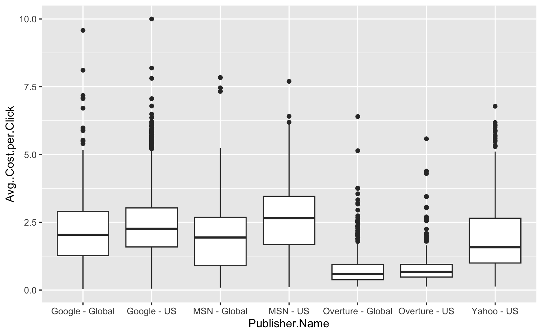
The box plot shows the average cost per click for different publishers, such as Google and Yahoo. It highlights:
-
The price publisher pays for each click varies greatly depending on the company whether the ads are run Globally or only in the United States.
-
Google generally charges more per click than MSN or Overture.
-
Overture frequently charges the lowest cost per click, in the United States.
-
The horizontal line in the center of each box indicates the median cost, higher the median more expensive the cost.
-
There are some cases where clicks are significantly less or more expensive than average.
-
Each publisher has outliers, with Google Global having especially expensive outliers.
-
The cost of clicks varies depending on the organization.
This data helps businesses in decide where to place their advertisements in order to achieve the highest return on investment.
# Visualization 2: Calculating Cost per Click per Publisher Name
publisher_cpc <- data %>%
  group_by(Publisher.Name) %>%
  summarize(Total_Cost = sum(Total.Cost), Total_Clicks = sum(Clicks), CPC = ifelse(Total_Clicks > 0, Total_Cost / Total_Clicks, 0)) %>%
  arrange(desc(CPC))

# Creating the bar chart for Cost per Click
ggplot(publisher_cpc, aes(x = reorder(Publisher.Name, -CPC), y = CPC)) +
  geom_bar(stat = "identity", fill = "steelblue") +
  theme(axis.text.x = element_text(angle = 45, hjust = 1)) +
  labs(x = "Publisher Name", y = "Cost per Click (CPC)", title = "Cost per Click by Publisher")
Output:
Visualization 2
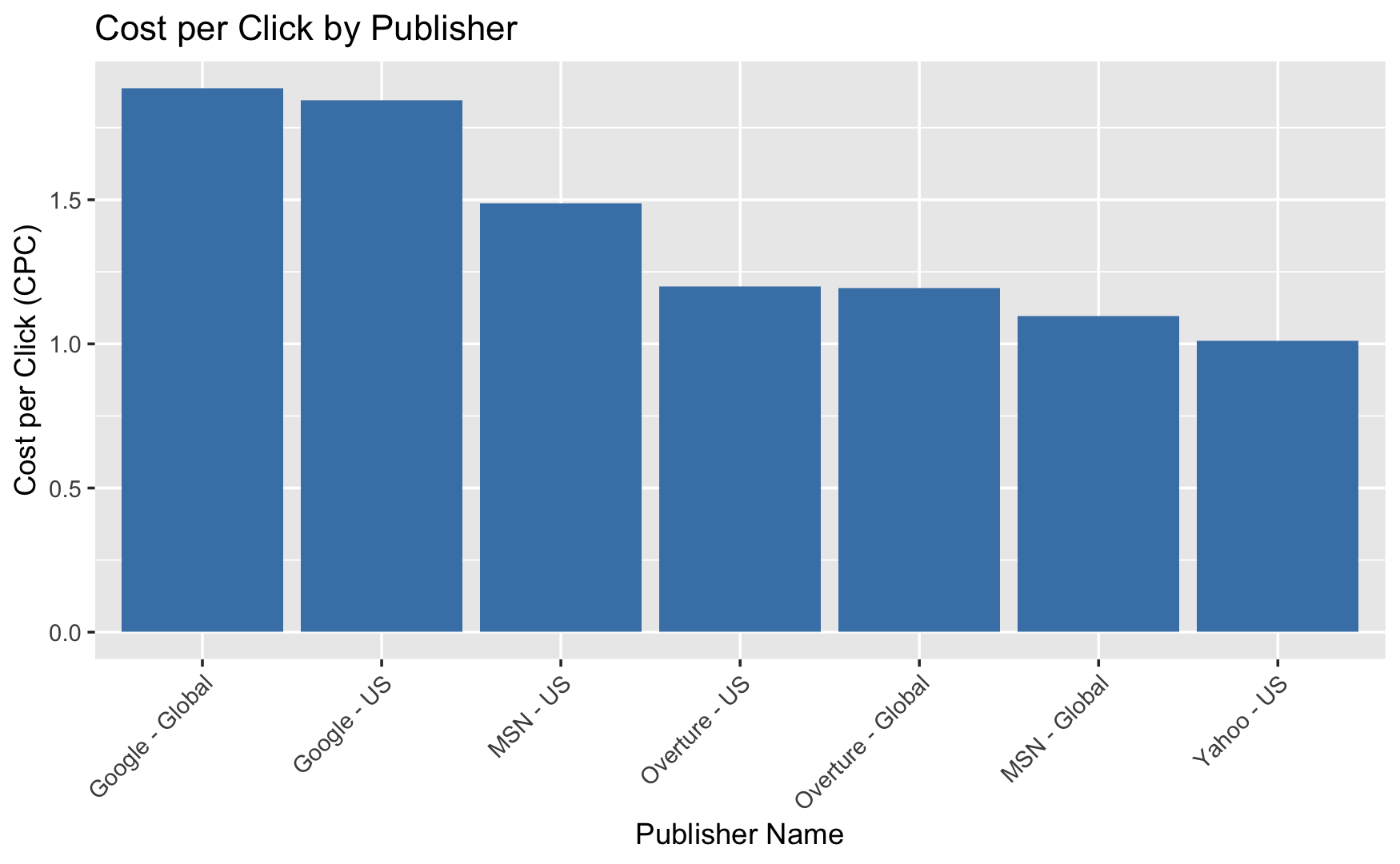
The bar chart shows average cost per click (CPC) for publishers. It highlights:
-
Google Global has the highest average cost-per-click, with more than 1.5 (CPC).
-
Google US follows closely with the second highest CPC.
-
MSN US has a somewhat high CPC, which is lower than the two Google categories.
-
CPCs for Overture US and MSN Global are similar, falling in the lower middle range.
-
Overture Global has a lower cost per click (CPC) than Overture US and MSN Global.
-
Yahoo US has the lowest CPC of the publishers listed.
The chart clearly shows CPC pricing differences amongst publishers that may influences marketers. Advertisers may select Yahoo US for the most cost-effective clicks. Google’s services, while more expensive, may have a wider reach or perceived value. This data can help advertisers in budgeting campaigns and selecting cost-effective platforms.
# Visualization 3: Aggregate and Sum Bookings by Publisher
agg_book <- aggregate(Total.Volume.of.Bookings ~ Publisher.Name, data = data, FUN = sum)
agg_book <- agg_book[order(-agg_book$Total.Volume.of.Bookings), ]

# Creating bar chart for publisher and the booking
ggplot(data = agg_book, aes(x = reorder(Publisher.Name, -Total.Volume.of.Bookings), y = Total.Volume.of.Bookings)) +
  geom_bar(stat = "identity") +
  labs(x = "Publisher Name", y = "Total Volume of Bookings", title = "Volume of Bookings for Various Publishers")
Output:
Visualization 3
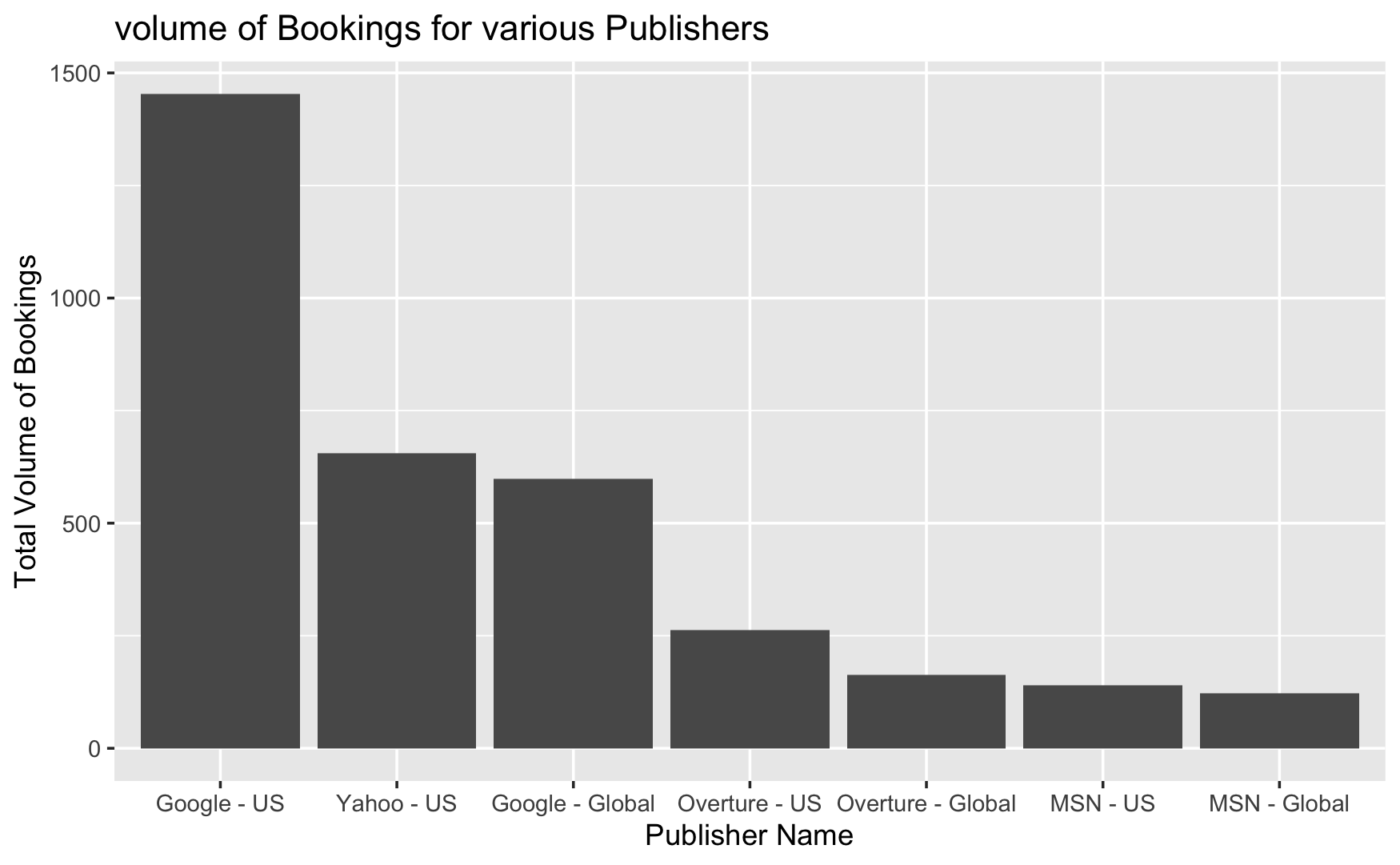
The bar chart shows the overall volume of bookings for various publishers. The graphic provides a simple way to compare booking volumes across different publishers and markets, representing that Google - US leads this statistic. It highlights:
-
Google - US has the largest overall volume of bookings, approaching 1500.
-
Yahoo - US comes in second, with slightly more than half the volume of Google - US.
-
Google - Global ranks third, with a somewhat lower overall volume than Yahoo - US.
-
Overture - US ranks fourth, closely followed by Overture - Global.
-
MSN - US and MSN - Global had the lowest total number of bookings among the listed publishers, with MSN - Global having the fewest.
In the bars for “US” market publishers are often higher than their “Global” competitors, which could indicate that these publishers perform better or have a stronger presence in the US market.
# Output 4: Count of Publishers
Publishers <- length(unique(data$Publisher.Name))
print(paste("Publishers:", Publishers))

# Visualization 4: Aggregate and Sum Clicks by Publisher
agg_clicks <- aggregate(Clicks ~ Publisher.Name, data = data, FUN = sum)
agg_clicks <- agg_clicks[order(-agg_clicks$Clicks), ]

# Bar chart for publisher and the clicks
ggplot(data = agg_clicks, aes(x = reorder(Publisher.Name, -Clicks), y = Clicks)) +
  geom_bar(stat = "identity", fill = "blue") +
  labs(x = "Publisher Name", y = "Clicks", title = "Clicks for Each Publisher")
Output:
Visualization 4
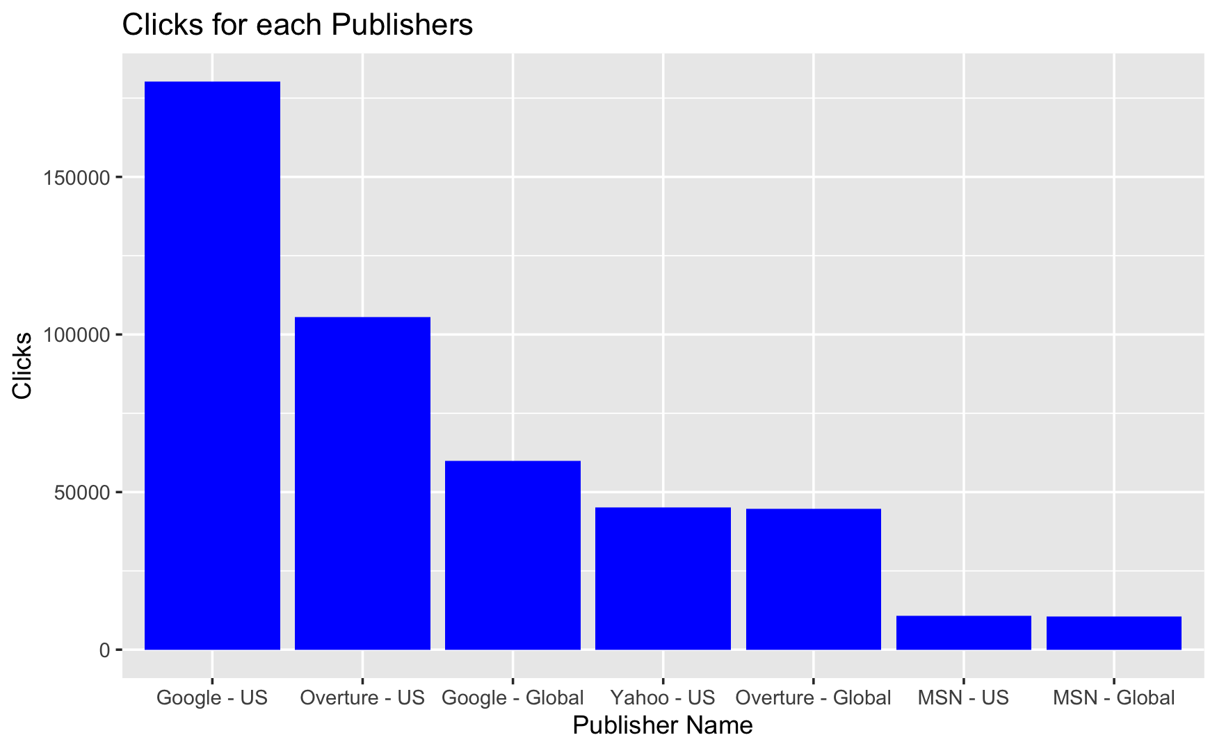
The bar chart shows the clicks for several publishers from both the US and global markets. Clicks are tracked for Google-US, Overture-US, Google-Global, Yahoo-US, Overture-Global, MSN-US, and MSN-Global. It highlights:
-
Google – US received the most clicks, with the bar reaching more than 150,000, showing a large lead over the other publishers.
-
Overture - US comes in second, but with fewer than two-thirds the number of clicks as Google - US.
-
Google - Global is close behind Overture - US, suggesting a large global presence.
-
Yahoo - US and Overture - Global have comparable click volumes, which are both lower than Google - Global but still significant.
-
MSN - US and MSN - Global had the fewest number of clicks, with MSN - Global having the least.
This could reveal numerous aspects, including Google’s dominance in the US market and the global success of these publishers. It also demonstrates the huge contrast in click volumes between marketplaces and publications.
# Visualization 5: Calculating the ratio of Total Volume of Bookings to Clicks for each publisher
publisher_cr <- data %>%
  group_by(Publisher.Name) %>%
  summarize(Total_Bookings = sum(Total.Volume.of.Bookings), Total_Clicks = sum(Clicks), Conversion_Rate = ifelse(Total_Clicks > 0, Total_Bookings / Total_Clicks, 0)) %>%
  arrange(desc(Conversion_Rate))

# Creating the bar chart for Conversion Rate
ggplot(publisher_cr, aes(x = reorder(Publisher.Name, -Booking_Click_Ratio),
                         y = Booking_Click_Ratio)) +
  geom_bar(stat = "identity", fill = "steelblue") +
  labs(x = "Publisher Name", y = "Bookings per Click Ratio",
       title = "Bookings per Click Ratio by Publisher")
Output:
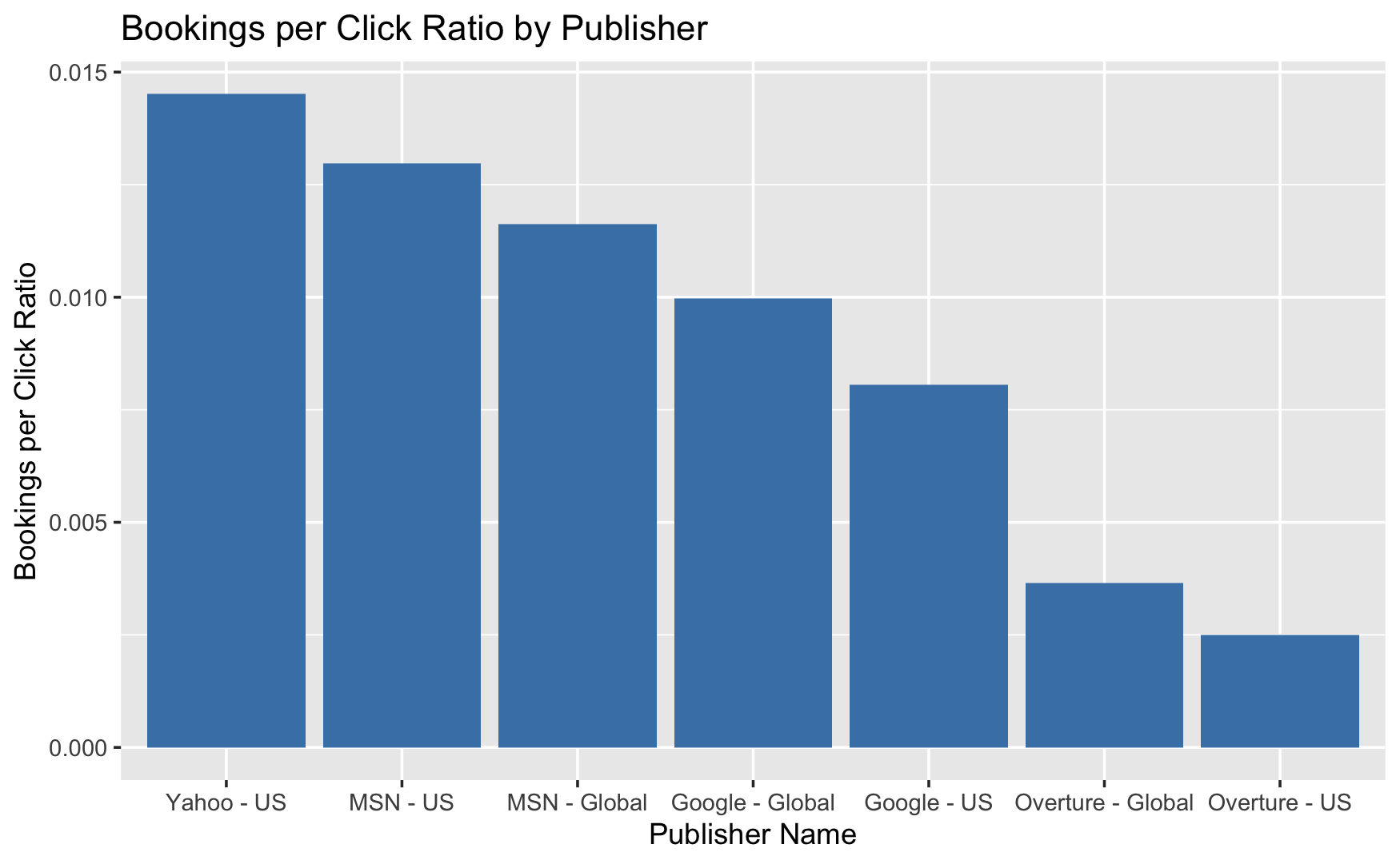
Visualization 5
The bar chart named “Bookings per Click Ratio by Publisher” that compares the efficiency of bookings to clicks across various publishers in both the US and global markets. It highlights:
-
Yahoo - US has the best bookings per click ratio, indicating that it converts the most clicks into bookings when compared to its click count.
-
MSN - US comes next, with a slightly lower ratio than Yahoo - US but still greater than the rest, demonstrating good market efficiency in the United States.
-
MSN - Global, Google - Global, and Google - US have successively lower ratios, showing that while they receive a lot of clicks, the conversion to bookings is not as great as Yahoo - US or MSN - US.
-
Overture - Global and Overture - US have the lowest bookings per click ratios, implying that they may require more clicks to obtain a booking than others.
This measure is frequently used to assess an ad publisher’s performance in turning clicks into bookings, with greater ratios being considered better. According to the bars, some publishers may be more effective globally, while others may flourish in the United States.
# Output 5

# Total clicks converted to Booking for each Publisher
conversion_rates <- data %>%
  group_by(Publisher.Name) %>%
  summarise(Total_Clicks = sum(Clicks, na.rm = TRUE),
            Total_Bookings = sum(Total.Volume.of.Bookings, na.rm = TRUE),
            Conversion_Rate = (Total_Bookings / Total_Clicks) * 100) %>%
  arrange(desc(Conversion_Rate))

# Display the conversion rates
print(conversion_rates)
| Publisher.Name | Total_Clicks | Total_Bookings | Conversion_Rate |
|---|---|---|---|
| Yahoo - US | 45198 | 656 | 1.4513917 |
| MSN - US | 10788 | 140 | 1.2977382 |
| MSN - Global | 10494 | 122 | 1.1625691 |
| Google - Global | 59918 | 598 | 0.9980306 |
| Google - US | 180208 | 1453 | 0.8062905 |
| Overture - Global | 44661 | 163 | 0.3649717 |
| Overture - US | 105541 | 263 | 0.2491923 |
Explanation
This code is created to give an overview of the rate at which each Publishers, clicks turns to booking. This shows how each cost the client pays for each click for every publisher turns to revenue to the client. Total bookings were divided by total clicks to show the rate clicks are converted. This shows how effective publishers have been able to push adverts to the right customers. This have been arranged in descending order for proper analysis. The results showed that Yahoo - US gave a higher conversion rate of 1.45%. Meaning that 1.45% of every click we pay for turns into booking which is the primary aim for business.
# Output 6

# Calculate Net Returns (Amount - Total Cost) by Publisher
net_returns_publisher <- data %>%
  group_by(Publisher.Name) %>%
  summarise(
    # Calculate net returns for each publisher
    Net_Returns = sum(as.numeric(Amount)) - sum(as.numeric(Total.Cost))
  ) %>%
  # Arranging in descending order of net returns for fast analysis
  arrange(desc(Net_Returns))

# Display Results
print(net_returns_publisher)
| Publisher.Name | Net_Returns |
|---|---|
| Google - US | 1316771.7 |
| Yahoo - US | 832648.2 |
| Google - Global | 559704.8 |
| Overture - US | 191429.1 |
| MSN - US | 165488.2 |
| Overture - Global | 129901.6 |
| MSN - Global | 128099.1 |
# Visualization 6

# Calculating ROI per Publisher Name
publisher_roi <- data %>%
  group_by(Publisher.Name) %>%
  summarize(Total_Amount = sum(Amount), Total_Cost = sum(Total.Cost),
            ROI = ifelse(Total_Cost > 0, (Total_Amount - Total_Cost) / Total_Cost, 0)) %>%
  arrange(desc(ROI))

# Creating the bar chart for ROI
ggplot(publisher_roi, aes(x = reorder(Publisher.Name, -ROI), y = ROI)) +
  geom_bar(stat = "identity", fill = "skyblue") +
  theme(axis.text.x = element_text(angle = 45, hjust = 1)) +
  labs(x = "Publisher Name", y = "ROI", title = "ROI by Publisher")
Output:
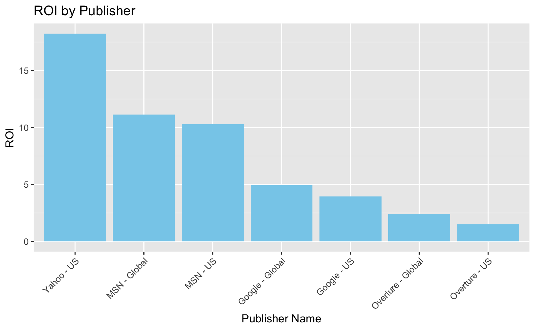
Visualization 6
The bar chart labelled “ROI by Publisher” that calculates the Return on Investment (ROI) for various publishers. It highlights:
-
Yahoo - US has the greatest ROI, with a number greater than 15, suggesting that investing in Yahoo’s US advertisements yields much larger returns than other publishers.
-
MSN - Global and MSN - US come next, with MSN - Global marginally outperforming MSN - US, indicating a good ROI for these areas.
-
Google - Global has a ROI of about 5, which is moderate compared to the others, whereas Google - US is slightly lower, indicating a poorer return per investment in these regions.
-
Overture - Global has a ROI that is around half that of Google, indicating inferior investment efficiency.
-
Overture - US has the lowest ROI on the chart, implying that investing in Overture’s US ads yields the lowest return compared to the others.
The chart indicates which publishes and markets may generate higher financial returns on advertising spend. Advertisers must take such data into account when developing marketing strategy.
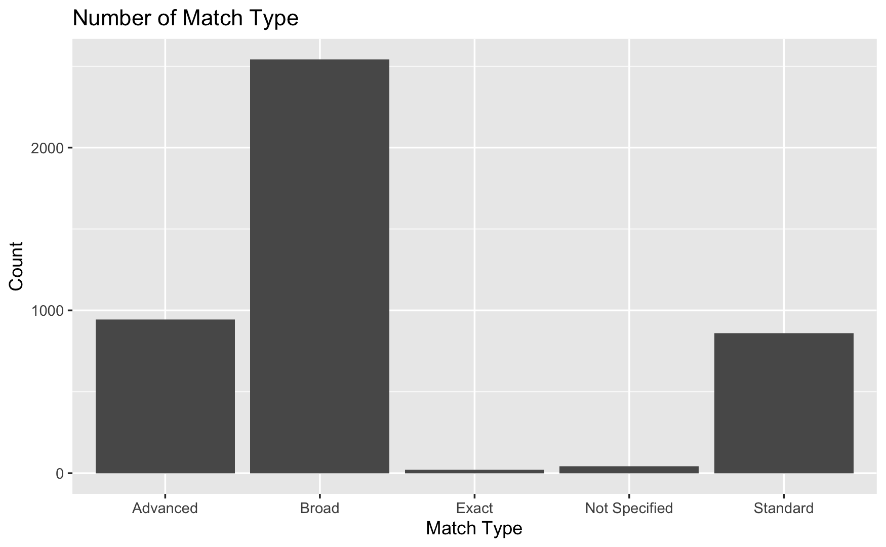
# Visualization 7

# Checking summary and the structure of the match type
summary(data$Match.Type)
str(data$Match.Type)

# Plotting histogram of match type for the keywords
# Creating a bar chart
mat_typ <- ggplot(data= data, aes(x= Match.Type))
mat_typ + geom_bar() +
  labs(x = "Match Type", y = "Count", title = "Number of Match Type")
Output:
# Visualization 8

# Creating a bar chart
rev<- ggplot(data= data, aes(x= Publisher.Name, y= Amount)) +
  geom_bar(stat="identity") +
  labs(x = "Publisher Name", y = "Amount", title = "")
rev

# Visualization 9

# Creating a bar chart
amt_spnd <- ggplot(data= data, aes(x= Publisher.Name, y= Total.Cost)) +
  geom_bar(stat="identity") +
  labs(x = "Match Type", y = "Count", title = "Number of Match Type")
amt_spnd

# Visualization 10

## word cloud
names(data)[names(data) == 'Keyword'] <- 'text'

wld_cld <- VCorpus(VectorSource(data$text))
wld_cld <- tm_map(wld_cld, content_transformer(tolower))  # convert to lower case
wld_cld <- tm_map(wld_cld, removePunctuation)             # remove punctuation
wld_cld <- tm_map(wld_cld, removeNumbers)                 # remove numbers
wld_cld <- tm_map(wld_cld, stripWhitespace)               # remove redundant spaces

tidy_text <- tidy(wld_cld)
tidy_text <- data %>%
  mutate(row = row_number()) %>%
  unnest_tokens(word, text)

print(colnames(tidy_text))
print(colnames(stop_words))

tidy_text <- tidy_text %>%
  anti_join(stop_words, by = "word")

word_freq <- tidy_text %>%
  count(word, sort = TRUE)
print(head(word_freq, 4))

wordcloud2(word_freq,
           color='random-light',
           shape = 'cloud',
           rotateRatio = 1)
Output:
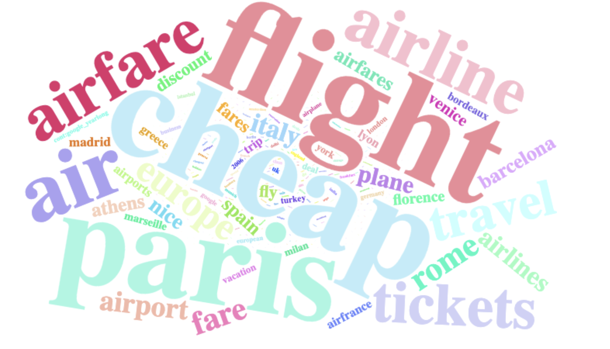
Visualization 10
The word cloud, which is a visual representation of text data in which the size of each word represents its frequency or relevance. Travel-related terms, notably flights and air travel, dominate this word cloud. Important findings from the word cloud:
-
The word “flight” and “cheap” are the most common, implying a heavy emphasis on low-cost air travel.
-
The titles of various European cities and countries, such as “France,” “Paris,” “Rome,” “Italy,” and “Europe,” reflect a concentration on this region.
-
Words like “Tickets,” “Fares,” “Airfare,” and “Discount” are also used frequently, highlighting the cost of air travel.
-
The appearance of the word “Airline” alongside specific cities shows that the data is related to searches or discussions regarding airlines that serve these areas.
-
The term “airport” and the names of specific cities denote a possible study of air travel routes or destinations.
Overall, the word cloud appears to indicate subjects connected to searching for or discussing economical flight.
# Output 8

# Defining a data frame named kayak_tab
kayak_tab <- data.frame(
  Search_Engine = "Kayak",
  Clicks = 2839,
  Media_Cost = 3567.13,
  Total_Bookings = 208,
  Avg_Ticket = 1123.53,
  Total_Revenue = 233694.00,
  Net_Revenue = 230126.87,
  stringsAsFactors = FALSE
)

# Display an interactive table with DT
datatable(kayak_tab, options = list(pageLength = 5, scrollX = TRUE))

# Display kayak data as a tabular output
print(kayak_tab)
| Search_Engine | Clicks | Media_Cost | Total_Bookings | Avg_Ticket | Total_Revenue | Net_Revenue |
|---|---|---|---|---|---|---|
| Kayak | 2839 | 3567.13 | 208 | 1123.53 | 233694 | 230126.9 |
# Output 9

# Calculate Cost Per Click for each publisher
Cost_per_Click_Publisher <- data %>%
  group_by(Publisher.Name) %>%
  summarise(
    Total_Cost = sum(as.numeric(Total.Cost), na.rm = TRUE),
    # Sum up clicks, also ignoring NA values
    Total_Clicks = sum(Clicks, na.rm = TRUE),
    # Calculate CPC; avoid division by zero by setting CPC to NA when no clicks are present
    Cost_Per_Click = ifelse(Total_Clicks > 0, Total_Cost / Total_Clicks, NA)
  ) %>%
  arrange(desc(Cost_Per_Click))

# Display the calculated Cost-Per_Click for each publisher
print(Cost_per_Click_Publisher)
| Publisher.Name | Total_Cost | Total_Clicks | Cost_Per_Click |
|---|---|---|---|
| Google - Global | 113007.35 | 59918 | 1.886033 |
| Google - US | 332410.22 | 180208 | 1.844592 |
| MSN - US | 16061.60 | 10788 | 1.488839 |
| Overture - US | 126512.53 | 105541 | 1.198705 |
| Overture - Global | 53318.48 | 44661 | 1.193849 |
| MSN - Global | 11498.05 | 10494 | 1.095678 |
| Yahoo - US | 45691.64 | 45198 | 1.010922 |
# Output 10
# Calculating metrics by Match Type
Match_type_metrics <- data %>%
  group_by(Match.Type) %>%
  summarise(
    Total_Clicks = sum(Clicks, na.rm = TRUE),
    Total_Impressions = sum(Impressions, na.rm = TRUE),
    Total_Bookings = sum(Total.Volume.of.Bookings, na.rm = TRUE),
    Conversion_Rate = (Total_Bookings / Total_Clicks) * 100
  ) %>%
  mutate(Conversion_Rate = ifelse(is.nan(Conversion_Rate), 0, Conversion_Rate)) # Replace NaN with 0 in case of division by zero

# Display the calculated metrics
print(Match_type_metrics)
| Match.Type | Total_Clicks | Total_Impressions | Total_Bookings | Conversion_Rate |
|---|---|---|---|---|
| Advanced | 88514 | 14809846 | 758 | 0.85636171 |
| Broad | 215044 | 4717206 | 1640 | 0.76263462 |
| Exact | 45294 | 236914 | 672 | 1.48364022 |
| Not Specified | 1070 | 592612 | 1 | 0.09345794 |
| Standard | 106886 | 19021090 | 324 | 0.30312670 |
Top three actionable insights
Through the analytically processes have extracted pivotal findings:
-
The expenditure analysis highlights that a significant portion of the search engine marketing budget is allocated to Google - Global and Google - US. These platforms, while generating the highest click-through (180,208 clicks) and booking volume, exhibit modest returns on investment (ROI)—4.95 for Google - Global and 3.96 for Google - US.It is suggested that the Finance and Marketing teams collaborate to refine the budget allocation for these platforms to enhance efficiency and optimize ROI.
-
An in-depth ROI analysis indicates a standout performance by Yahoo as the search engine marketing channel, yielding an ROI of 18.22. Despite only 7.63% of the search engine marketing budget being directed towards Yahoo, it delivers the most favorable conversion rate at 1.45 and maintains the lowest cost per click at $1.01. It is advised to redirect funds from Google to Yahoo, anticipating improved outcomes without escalating the overall marketing spend.
-
The keyword strategy assessment reveals that ‘Broad’ match type predominates the usage, with 45,294 instances leading to 236,914 impressions and 672 bookings. This match type achieves the highest conversion rate at 1.48 compared to its counterparts. Data underscores the strategic advantage of targeting precise keywords to maximize conversion efficiency. The Marketing team is encouraged to utilize the Word Cloud for a granular analysis to determine the most impact keywords for our campaigns, prioritizing high-conversion keywords and eliminating or reducing spending on low-performing keywords.
Part II: Model Development in Python
1. Introduction
This part focuses on using the preprocessed and cleaned dataset from the R analysis to develop predictive models in Python. The goal is to forecast the number of clicks for future digital marketing campaigns.
2. Data Preparation and Feature Engineering
The data preparation phase involved several steps to clean and transform the dataset to make it suitable for modeling. Key steps included:
- Data Cleaning: Removing non-numeric characters and handling missing values.
- Log Transformations: Applying logarithmic transformations to normalize skewed distributions.
- Feature Engineering: Creating new features from existing data to improve model performance.
Data Cleaning
import pandas as pd
import numpy as np
import seaborn as sns
import matplotlib.pyplot as plt
from scipy.stats import yeojohnson
import re
from sklearn.feature_extraction.text import TfidfVectorizer
from sklearn.preprocessing import StandardScaler
import nltk
from sklearn.metrics import mean_squared_error
from sklearn.tree import DecisionTreeRegressor
from sklearn.ensemble import GradientBoostingRegressor, RandomForestRegressor
from sklearn.neural_network import MLPRegressor
from sklearn.model_selection import train_test_split, RandomizedSearchCV

# Load the datasets
df_train = pd.read_csv('./datasets/train.csv', index_col='entry_id')
df_test = pd.read_csv('./datasets/test.csv', index_col='entry_id')

# Concatenate datasets for cleaning and feature engineering
df_train['set'] = 'Not Kaggle'
df_test['set'] = 'Kaggle'
df_full = pd.concat([df_train, df_test])

# Rename columns for consistency
df_full = df_full.rename(columns={
    'Publisher Name': 'Publisher_Name',
    'Keyword': 'Keyword',
    'Match Type': 'Match_Type',
    'Campaign': 'Campaign',
    'Keyword Group': 'Keyword_Group',
    'Category': 'Category',
    'Bid Strategy': 'Bid_Strategy',
    'Status': 'Status',
    'Search Engine Bid': 'Search_Engine_Bid',
    'Impressions': 'Impressions',
    'Avg. Pos.': 'Avg_Pos',
    'Avg. Cost per Click': 'Avg_Cost_per_Click',
    'Clicks': 'Clicks',
    'set': 'set'
})

# Data cleaning: Convert 'Search Engine Bid', 'Avg. Cost per Click', 'Clicks', and 'Impressions' to numeric
df_full['Search_Engine_Bid'] = pd.to_numeric(df_full['Search_Engine_Bid'].str.replace('[\$,]', '', regex=True), errors='coerce')
df_full['Avg_Cost_per_Click'] = pd.to_numeric(df_full['Avg_Cost_per_Click'].str.replace('[\$,]', '', regex=True), errors='coerce')
df_full['Clicks'] = pd.to_numeric(df_full['Clicks'].str.replace(',', ''), errors='coerce')
df_full['Impressions'] = pd.to_numeric(df_full['Impressions'].str.replace(',', ''), errors='coerce')

## Missing Value Imputation ##
df_full.isnull().describe()
df_full.isnull().sum(axis = 0)

# looping to flag features with missing values
for col in df_full:

    # creating columns with 1s if missing and 0 if not
    if df_full[col].isnull().astype(int).sum() > 0:
        df_full['m_'+col] = df_full[col].isnull().astype(int)
df_full = df_full.drop(columns=['m_Clicks'])

# subsetting for mv features
mv_flag_check = df_full[ ['Match_Type'     , 'm_Match_Type',
                          'Bid_Strategy' , 'm_Bid_Strategy'] ]

# checking results - feature comparison
mv_flag_check.sort_values(by = ['m_Match_Type', 'm_Bid_Strategy'],
                          ascending = False).head(n = 10)
#Now, we are going to filter just the Campaign and Publisher Namer that null values matched before
filtered_data_1 = df_full[(df_full['Publisher_Name'].isin(['Google - Global', 'Google - US'])) & (df_full['Campaign'].isin(['Air France Global Campaign', 'Google_Yearlong 2006']))]
filtered_data_1.groupby(['Match_Type', 'Publisher_Name', 'Campaign']).Clicks.count()
#As we can see, the Broad Match Type fits perfectly with the Publisher Name and Campaign of Match Type null values

# imputing Match_Type
df_full['Match_Type'].fillna(value   = 'Broad',
                             inplace = True)
#Check the correct imputation
df_full[ ['Match_Type', 'm_Match_Type'] ][df_full['m_Match_Type'] == 1].head(n = 10)

#Let's see the same behaviour with Bid Strategy, but first, we are going to clean some misspelling
df_full['Bid_Strategy'].value_counts()
#For instance, Position 1 -2 Target and Position 1-2 Target are the same, just a space of diff
#The same with Position 1-4 Bid Strategy and Postiion 1-4 Bid Strategy, that has double ii.

# Defining a dictionary to map misspelled values to their corrected versions
corrections = {
    'Position 1 -2 Target': 'Position 1-2 Target',
    'Postiion 1-4 Bid Strategy': 'Position 1-4 Bid Strategy',
    'Position 1- 3': 'Position 1-3',
    'Pos 3-6': 'Position 3-6'
}

# Apply the corrections using the replace method
df_full['Bid_Strategy'] = df_full['Bid_Strategy'].replace(corrections)

# Verify the changes
print(df_full['Bid_Strategy'].value_counts())

# Creating a dictionary with rules to replace null values in Bid_Strategy
replacement_dict = {
    ('Google - US', 'Air France Branded', 'uncategorized', 'Live'): 'Position 1-2 Target',
    ('Google - US', 'Air France Branded', 'uncategorized', 'Paused'): 'Position 1-2 Target',
    ('Overture - US','Unassigned','bordeaux','Paused'):'Position 1-4 Bid Strategy',
    ('Overture - US','Unassigned','flight','Unavailable'):'Position 1-4 Bid Strategy',
    ('Google - US','Business Class','uncategorized','Live'):'Position 2-5 Bid Strategy',
    ('Google - US','French Destinations','uncategorized','Live'):'Position 2-5 Bid Strategy',
    ('Google - US','French Destinations','uncategorized','Paused'):'Position 2-5 Bid Strategy',
    ('Google - US','Geo Targeted Seattle','uncategorized','Paused'):'Position 2-5 Bid Strategy',
    ('Google - US','Paris & France Terms','uncategorized','Live'):'Position 2-5 Bid Strategy',
    ('Overture - US','Unassigned','airfrance','Paused'):'Position 2-5 Bid Strategy',
    ('Overture - US','Unassigned','airfrance','Unavailable'):'Position 2-5 Bid Strategy',
    ('Overture - US','Unassigned','france','Paused'):'Position 2-5 Bid Strategy',
    ('Overture - US','Unassigned','lyon','Paused'):'Position 2-5 Bid Strategy',
    ('Overture - US','Unassigned','marseille','Paused'):'Position 2-5 Bid Strategy',
    ('Overture - US','Unassigned','nice','Paused'):'Position 2-5 Bid Strategy',
    ('Overture - US','Unassigned','paris','Paused'):'Position 2-5 Bid Strategy',
    ('Google - US','Paris & France Terms','uncategorized','Paused'):'Position 3-6',
    ('Google - US','Paris & France Terms','uncategorized','Unavailable'):'Position 3-6',
    'Google - Global': 'Position 1-3',
    'Overture - Global': 'Position 1-2 Target'
}
# imputing Bid_Strategy
for conditions, bid_strategy in replacement_dict.items():
    if isinstance(conditions, tuple):  # Si son condiciones detalladas
        df_full.loc[(df_full['Publisher_Name'] == conditions[0]) &
                    (df_full['Campaign'] == conditions[1]) &
                    (df_full['Category'] == conditions[2]) &
                    (df_full['Status'] == conditions[3]) &
                    (df_full['Bid_Strategy'].isnull()), 'Bid_Strategy'] = bid_strategy
    else:  # Si es un caso simplificado
        df_full.loc[df_full['Publisher_Name'] == conditions, 'Bid_Strategy'] = df_full['Bid_Strategy'].fillna(bid_strategy)

# imputing last Bid_Strategy null values
df_full['Bid_Strategy'].fillna(value   = 'Position 5-10 Bid Strategy',
                             inplace = True)
#Check the correct imputation
df_full[ ['Bid_Strategy', 'm_Bid_Strategy'] ][df_full['m_Bid_Strategy'] == 1].head(n = 10)
Log Transformations and Feature Engineering
# Apply logarithmic transformations to normalize distributions
df_full['log_Clicks'] = np.log1p(df_full['Clicks'])
df_full['log_Impressions'] = np.log1p(df_full['Impressions'])
df_full['log_Avg_Pos'] = np.log1p(df_full['Avg_Pos'])
df_full['log_Avg_Cost_per_Click'] = np.log1p(df_full['Avg_Cost_per_Click'])

# Apply Yeo-Johnson transformation for better normalization
df_full['YeoJohnson_Clicks'], _ = yeojohnson(df_full['Clicks'])
df_full['YeoJohnson_Impressions'], _ = yeojohnson(df_full['Impressions'])
df_full['YeoJohnson_Avg_Pos'], _ = yeojohnson(df_full['Avg_Pos'])
df_full['YeoJohnson_Avg_Cost_per_Click'], _ = yeojohnson(df_full['Avg_Cost_per_Click'])

# Create new features
df_full['Impressions_Bid'] = df_full['Impressions'] * df_full['Search_Engine_Bid']
df_full['AvgPos_Bid'] = df_full['Avg_Pos'] * df_full['Search_Engine_Bid']
df_full['Keyword_Length'] = df_full['Keyword'].apply(len)
# placeholder variables
df_full['has_Search_Engine_Bid'] = 0

old_cat = ['Outside Western Europe', 'Geo Targeted Cincinnati', 'General Terms']

# Replacing
df_full['Campaign'] = df_full['Campaign'].replace(old_cat, 'Others')

# iterating over each original column to
# change values in the new feature columns
for index, value in df_full.iterrows():


    # Solar Radiation
    if df_full.loc[index, 'Search_Engine_Bid'] > 0:
        df_full.loc[index, 'has_Search_Engine_Bid'] = 1

# analyzing (Pearson) correlations
df_corr = df_full.corr(method = 'pearson',numeric_only = True ).round(2)

df_corr.loc[ : , ['Clicks', 'log_Clicks','YeoJohnson_Clicks'] ].sort_values(by = 'Clicks',
                                                                ascending = False)

# one hot encoding categorical variables
one_hot_Publisher_Name = pd.get_dummies(df_full['Publisher_Name'])
one_hot_Match_Type = pd.get_dummies(df_full['Match_Type'])
one_hot_Campaign = pd.get_dummies(df_full['Campaign'])
one_hot_Bid_Strategy = pd.get_dummies(df_full['Bid_Strategy'])
one_hot_Bid_Status = pd.get_dummies(df_full['Status'])

# dropping categorical variables after they've been encoded
df_full = df_full.drop('Publisher_Name', axis = 1)
df_full = df_full.drop('Match_Type', axis = 1)
df_full = df_full.drop('Campaign', axis = 1)
df_full = df_full.drop('Bid_Strategy', axis = 1)
df_full = df_full.drop('Status', axis = 1)

# joining codings together
df_full = df_full.join([one_hot_Publisher_Name,one_hot_Match_Type,one_hot_Campaign,one_hot_Bid_Strategy,one_hot_Bid_Status])

# saving new columns
new_columns = df_full.columns

# Define ranges for 'Avg. Pos.'
bins = [0, 1, 2, 3, 4, 5, float('inf')]
labels = ['1st', '2nd', '3rd', '4th', '5th', 'Above 5th']

# New feature: AvgPos_Category
df_full['AvgPos_Category'] = pd.cut(df_full['Avg_Pos'], bins=bins, labels=labels, include_lowest=True)

#Now, we are going to clean the keywords from special characters
def clean_keyword(keyword):
    # Delete special characters
    keyword_clean = re.sub(r'[^a-zA-Z0-9\s]', ' ', str(keyword))
    # Lowercase transformation
    keyword_clean = keyword_clean.lower()
    return keyword_clean

# Applying the function to 'Keyword' column
df_full['Keyword_Cleaned'] = df_full['Keyword'].apply(clean_keyword)

# Checking the dataset
df_full[['Keyword', 'Keyword_Cleaned']].tail(100)

df_full['Keyword_Length'] = df_full['Keyword_Cleaned'].apply(len)

#Downloading stopwords
nltk.download('stopwords')

#  Initialize the TF-IDF vectorizer with optional parameters
tfidf_vectorizer = TfidfVectorizer(max_features=1000,stop_words=stopwords.words('english'))  # Puedes ajustar 'max_features' según sea necesario
tfidf_matrix = tfidf_vectorizer.fit_transform(df_full['Keyword_Cleaned'])

# Converting in dataframe
tfidf_df = pd.DataFrame(tfidf_matrix.toarray(), columns=tfidf_vectorizer.get_feature_names_out())

# Checking the dataframe
tfidf_df.head()

#Merging the tfidf_df dataset with the df_full dataset
tfidf_df.index = df_full.index
df_full = pd.concat([df_full,tfidf_df], axis=1)
df_full = df_full.drop('Keyword', axis = 1)
df_full = df_full.drop('Keyword_Cleaned', axis = 1)
#Encoding the column 'Category' using the Clicks means
mean_encoding = df_full.groupby('Category')['Clicks'].mean()
df_full['Category'] = df_full['Category'].map(mean_encoding)
#Encoding the column 'Keyword_Group' using the Clicks means
mean_encoding_keyword_group = df_full.groupby('Keyword_Group')['Clicks'].mean()
df_full['Keyword_Group'] = df_full['Keyword_Group'].map(mean_encoding_keyword_group)
# one hot encoding categorical variables
one_hot_AvgPos_Category = pd.get_dummies(df_full['AvgPos_Category'])

# dropping categorical variables after they've been encoded
df_full = df_full.drop('AvgPos_Category', axis = 1)

# creating a (Pearson) correlation matrix
df_corr = df_full.corr(numeric_only = True).round(2)


# printing (Pearson) correlations with Clicks
df_corr.loc[ : , ['Clicks', 'log_Clicks', 'YeoJohnson_Clicks'] ].sort_values(by = 'Clicks',
                                                                ascending = False)
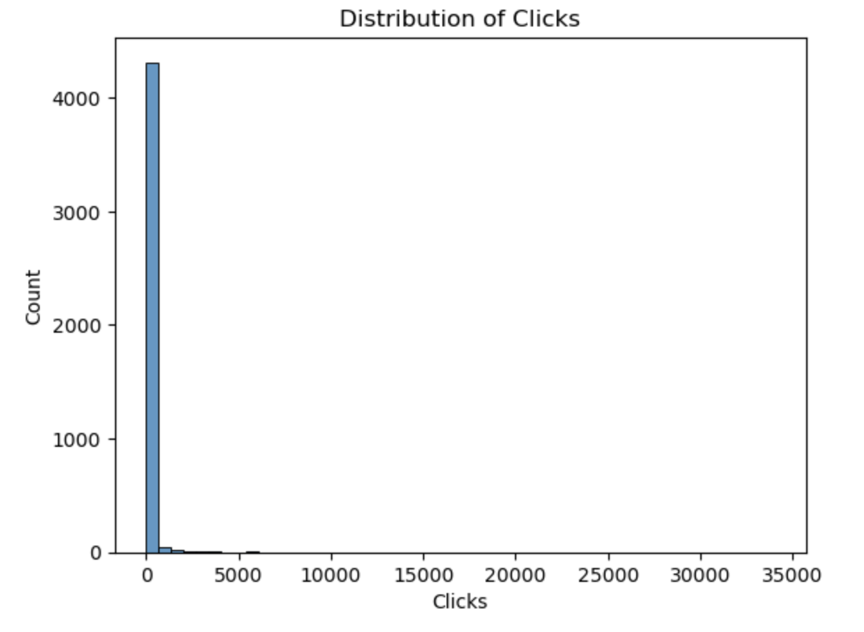
3. Exploratory Data Analysis (EDA)
Distribution of Clicks
# Plot the distribution of clicks
sns.histplot(data=df_full, x="Clicks", bins=50)
plt.title("Distribution of Clicks")
plt.xlabel("Clicks")
plt.ylabel("Count")
plt.show()
Output:
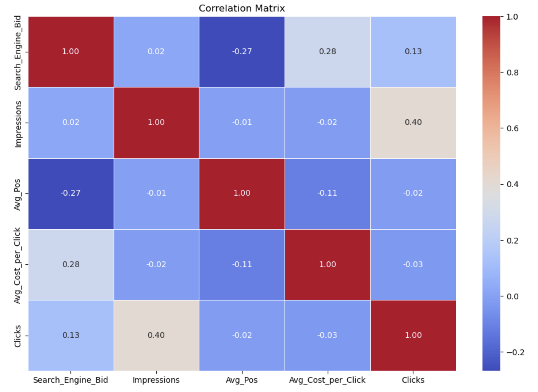
Correlation Matrix
# Compute and plot the correlation matrix
df_corr = df_full.corr(method='pearson')
plt.figure(figsize=(12, 8))
sns.heatmap(df_corr, annot=True, fmt=".2f", cmap='coolwarm', cbar=True, linewidths=0.5)
plt.title('Correlation Matrix')
plt.show()
Output:
4. Standardization
## Standardization ##

# preparing explanatory variable data
df_full_data   = df_full.drop(['Clicks',
                               'log_Clicks',
                               'YeoJohnson_Clicks',
                                'set'],
                                axis = 1)


# preparing the target variable
df_full_target = df_full.loc[ : , ['Clicks',
                               'log_Clicks', 'YeoJohnson_Clicks',
                                   'set']]

# INSTANTIATING a StandardScaler() object
scaler = StandardScaler()


# FITTING the scaler with the data
scaler.fit(df_full_data)


# TRANSFORMING our data after fit
x_scaled = scaler.transform(df_full_data)


# converting scaled data into a DataFrame
x_scaled_df = pd.DataFrame(x_scaled)


# checking the results
x_scaled_df.describe(include = 'number').round(decimals = 2)

# adding labels to the scaled DataFrame

#x_scaled_df = pd.DataFrame(x_scaled_df, index=df_full_data.index, columns=df_full_data.columns)
x_scaled_df.columns = df_full_data.columns
#  Checking pre- and post-scaling of the data
print(f"""
Dataset BEFORE Scaling
----------------------
{np.var(df_full_data)}


Dataset AFTER Scaling
----------------------
{np.var(x_scaled_df)}
""")
x_scaled_df.index = df_full_target.index
df_full = pd.concat([x_scaled_df, df_full_target], axis=1)

## parsing out testing data (needed for later) ##

# dataset for kaggle
kaggle_data = df_full[ df_full['set'] == 'Kaggle' ].copy()


# dataset for model building
df = df_full[ df_full['set'] == 'Not Kaggle' ].copy()


# dropping set identifier (kaggle)
kaggle_data.drop(labels = 'set',
                 axis = 1,
                 inplace = True)


# dropping set identifier (model building)
df.drop(labels = 'set',
        axis = 1,
        inplace = True)

# Excluding columns
exclude_columns = ['Clicks','YeoJohnson_Clicks','YeoJohnson_Impressions','boxcox_Impressions','Impressions']


# Choosing my x_features
x_features = [column for column in df.columns if column not in exclude_columns]
x_features
5. Model Development
We experimented with various regression models to find the best predictor for campaign clicks. The models included:
- Decision Tree Regressor
- Gradient Boosting Regressor
- Elastic Net
- Ridge Regression
- Lasso Regression
- K-Nearest Neighbors
- Random Forest Regressor
- MLP Regressor
Model Training and Evaluation
# Split data into training and testing sets
#!###########################!#
#!# choose your x-variables #!#
#!###########################!#
x_features = ['log_Impressions','Keyword_Group',
 'Category','Impressions_Bid', 'Air France Branded','Exact','Keyword_Length','Position 5-10 Bid Strategy',
 'Search_Engine_Bid','Impressions','log_Avg_Cost_per_Click', 'YeoJohnson_Avg_Pos','Broad','air','airfrance',
              'travel','Standard','Position 1-4 Bid Strategy','flight','flights','france','paris','Clicks']
# this should be a list


## ########################### ##
## DON'T CHANGE THE CODE BELOW ##
## ########################### ##

# removing non-numeric columns and missing values
df = df[x_features].copy().select_dtypes(include=[int, float]).dropna(axis = 0)


# prepping data for train-test split
x_data = df.drop(labels = y_variable,
                 axis   = 1)

y_data = df[y_variable]


# train-test split (to validate the model)
x_train, x_test, y_train, y_test = train_test_split(x_data,
                                                    y_data,
                                                    test_size    = 0.25,
                                                    random_state = 702 )


# Train and evaluate models
models = {
    "Decision Tree": DecisionTreeRegressor(max_depth=4, min_samples_leaf=25, random_state=702),
    "Gradient Boosting": GradientBoostingRegressor(n_estimators=390, learning_rate=0.1, max_depth=3, min_samples_leaf=25, random_state=702),
    "Ridge": Ridge(alpha=10.0, random_state=702),
    "Lasso": Lasso(alpha=1.0, random_state=702),
    "Elastic Net": ElasticNet(alpha=0.5, random_state=702),
    "KNN": KNeighborsRegressor(n_neighbors=5),
    "Random Forest": RandomForestRegressor(n_estimators=100, random_state=702),
    "MLP Regressor": MLPRegressor(hidden_layer_sizes=(100, 50), activation='relu', solver='adam', random_state=702)
}

for name, model in models.items():
    model.fit(x_train, y_train)
    y_pred = model.predict(x_test)
    train_score = model.score(x_train, y_train)
    test_score = model.score(x_test, y_test)
    rmse = np.sqrt(mean_squared_error(y_test, y_pred))
    print(f"{name} - Train Score: {train_score:.4f}, Test Score: {test_score:.4f}, RMSE: {rmse:.4f}")
Hyperparameter Tuning
Decision Tree Regressor
param_grid = {
    'criterion': ["squared_error", "friedman_mse", "absolute_error", "poisson"],
    'splitter': ["best", "random"],
    'max_depth': np.arange(1, 11),
    'min_samples_leaf': np.arange(0, 25, 5)
}

tuned_tree = DecisionTreeRegressor()
tuned_tree_cv = RandomizedSearchCV(estimator=tuned_tree, param_distributions=param_grid, cv=5, n_iter=10, random_state=702)
tuned_tree_cv.fit(x_data, y_data)

print("Tuned Parameters:", tuned_tree_cv.best_params_)
print("Tuned Training Score:", tuned_tree_cv.best_score_.round(4))
GradientBoosting Regressor
# declaring a hyperparameter space
learning_rate_range = np.linspace(0.01, 0.2, 20) # Experimenta con diferentes rangos y valores
n_estimators_range = np.arange(100, 1000, 100)
max_depth_range = np.arange(3, 10, 1)
min_samples_split_range = np.arange(2, 10, 1)
min_samples_leaf_range = np.arange(1, 10, 1)
max_features_range = ['auto', 'sqrt', 'log2', None]


# creating a hyperparameter grid
param_grid = {'learning_rate': learning_rate_range,
                'n_estimators': n_estimators_range,
                'max_depth': max_depth_range,
                'min_samples_split': min_samples_split_range,
                'min_samples_leaf': min_samples_leaf_range,
                'max_features': max_features_range}


# INSTANTIATING the model object without hyperparameters
tuned_gbr = GradientBoostingRegressor()


# RandomizedSearchCV object
tuned_gbr_cv = RandomizedSearchCV(estimator             = tuned_gbr, #model
                                   param_distributions   = param_grid, #hyperparameter ranges
                                   cv                    = 5,    #folds
                                   n_iter                = 10, #how many models to build
                                   random_state          = 702)


# FITTING to the FULL DATASET (due to cross-validation)
tuned_gbr_cv.fit(x_data, y_data)


# printing the optimal parameters and best score
print("Tuned Parameters  :", tuned_gbr_cv.best_params_)
print("Tuned Training AUC:", tuned_gbr_cv.best_score_.round(4))
MLPRegressor
# declaring a hyperparameter space
hidden_layer_sizes_range = [(50,), (100,), (100, 50)]
activation_range = ['relu']
solver_range = ['adam']
alpha_range = [0.0001, 0.001, 0.01]
learning_rate_range = ['constant', 'invscaling']
max_iter_range = [100, 200, 300]

# creating a hyperparameter grid
param_grid = {'hidden_layer_sizes': hidden_layer_sizes_range,
              'activation': activation_range,
              'solver': solver_range,
              'alpha': alpha_range,
              'learning_rate': learning_rate_range,
              'max_iter': max_iter_range}


# INSTANTIATING the model object without hyperparameters
mlp_reg = MLPRegressor()


# RandomizedSearchCV object
mlp_reg_cv = RandomizedSearchCV(estimator             = mlp_reg, #model
                                   param_distributions   = param_grid, #hyperparameter ranges
                                   cv                    = 5,    #folds
                                   n_iter                = 5,
                                   n_jobs                =-1,
                                   random_state          = 702)


# FITTING to the FULL DATASET (due to cross-validation)
mlp_reg_cv.fit(x_data, y_data)


# printing the optimal parameters and best score
print("Tuned Parameters  :", mlp_reg_cv.best_params_)
print("Tuned Training AUC:", mlp_reg_cv.best_score_.round(4))
| Model | RMSE |
|---|---|
| DecisionTree | 510.1588 |
| GradientBoostin | 331.5624 |
| Elastic Net | 375.4851 |
| Ridge | 484.5401 |
| Lasso | 482.8705 |
| Random Forest | 909.2221 |
| MLPRegressor | 570.0746 |
6. Conclusion
After evaluating multiple models, the Gradient Boosting Regressor emerged as the best performer with the highest accuracy and generalization capability. The final model provides valuable insights into the key factors influencing campaign clicks, which can help optimize future digital marketing strategies for Air France.
Final Model Performance
The tuned Gradient Boosting Regressor provided the best performance with the following parameters:
- Learning Rate: 0.16
- Number of Estimators: 900
- Max Depth: 3
- Min Samples Split: 9
- Min Samples Leaf: 2
- Max Features: ‘log2’
The final RMSE for the model is significantly lower, indicating improved prediction accuracy.
Final Conclusion
This project successfully developed a predictive model for forecasting clicks on Air France’s digital marketing campaigns. The analysis in R provided essential data cleaning and transformation, while the Python modeling section utilized advanced machine learning techniques to achieve accurate predictions.
Final Answer to the Business Question: The developed model can accurately predict the number of clicks for digital marketing campaigns, enabling Air France to optimize their advertising spend and improve campaign performance.
Bibliography
- Kellogg School of Management Business Case:
- Source: Kellogg School of Management
-
Beattie, A. (2024, 2 28). ROI: Return on Investment Meaning and Calculation. Investopedia. Retrieved from Investopedia
-
Lay, D. (n.d.). A Guide To Data Driven Decision Making: What It Is, Its Importance, & How To Implement It. Retrieved from tableau
- Ooi, J. (2023, 08 18). The Importance of Keyword Research in SEM: Maximizing Your Online Visibility. Retrieved from nightowl
This project is part of the Business Challenge II within the master’s program in Business Analytics at Hult International Business School and is part of an internal class competition on Kaggle.